As a result of a long-term collaboration, MathWorks Inc. and embotech AG developed a MATLAB® plugin for FORCESPRO. Users are now able to use the FORCESPRO solver in MATLAB® and Simulink® from within the MATLAB® Model Predictive Control Toolbox.
The plugin leverages the powerful design capabilities of the Model Predictive Control Toolbox™ and the computational performance of FORCESPRO.
Starting from FORCESPRO 2.0, toolbox users can now easily define challenging control problems and solve long-horizon MPC problems more efficiently.
Model Predictive Control Toolbox™ provides functions, an app, and Simulink® blocks for designing and simulating model predictive controllers. The toolbox enables users to readily specify plant and disturbance models, horizons, constraints, and weights. User-friendly control design capabilities of Model Predictive Control Toolbox™, combined with the powerful numerical algorithms of FORCESPRO, enables code deployment of the FORCESPRO solver on real-time hardware from within MATLAB® and Simulink®, in addition to the QP solvers shipped by MathWorks.
The new FORCESPRO interface comes with various features such as Simulink blocks that can generate code runnable on embedded targets such as dSPACE.
The parameters of the MPC algorithm, such as plant and disturbance model, prediction horizon, constraints and move-blocking strategy can be specified directly.
The toolbox enables users to run closed-loop simulations and evaluation of controller performance. User-friendly MPC design capabilities are combined with the powerful numerical algorithms of FORCESPRO. This combination of the Model Predictive Control Toolbox™ and FORCESPRO enables code deployment on real-time hardware.
The generated code is highly optimized for fast computations and low memory footprint.
This interface is provided with all variants of FORCESPRO, starting with Variant S. It is compatible from MATLAB R2018b onwards.
The plugin mainly consists of the three following MATLAB commands which are described in details in this chapter:
mpcToForces for generating a FORCESPRO solver from an MPC object designed by the Model Predictive Control Toolbox
mpcmoveForces for calling the generated solver on a specific linear time-invariant (LTI) MPC problem instance
mpcmoveAdaptiveForces for calling the generated solver on a specific adaptive or time-varying MPC problem instance
mpcCustomSolver for using the FORCESPRO dense QP solver as a custom solver
An auxiliary file is also exposed to the users for generating different solvers options, namely mpcToForcesOptions.
The following MPC features are supported:
Continuous and discrete time plant models
Move blocking
Measured disturbances
Unmeasured disturbances
Disturbance and noise models
Uniform or time-varying weights on outputs, manipulated variables, manipulated variables rates and a global slack variable
Uniform or time-varying bounds on outputs, manipulated variables and manipulated variables rates
Soft constraints
Signal previewing on reference and measured disturbances
Scale factors
Nominal values
Online updates of weights and constraints
Built-in and custom state estimators
Adaptive MPC and LTV MPC where plant model changes online (only available using sparse QP)
Currently, convex quadratic programs are supported by the MATLAB plugin. The current limitations of the plugin are the following:
Mixed input-output constraints are not covered
Off-diagonal terms on the hessian of the objective cannot be implemented
Unconstrained problems are not supported
No single-precision solvers, only double precision currently
The plugin converts an MPC object (weights, bounds, horizons, prediction model) into a quadratic program (QP) formulated via the FORCESPRO API. One key design decision is to choose the decision variables in the quadratic program.
There are two classic choices and they lead to two different formulations:
Dense QP, where only the manipulated variables \(MV\) or \(\Delta{}MV\) are decision variables. In this case, the hessian and linear constraints matrices are stored as dense matrices.
Sparse QP, where \(MV\), \(\Delta{}MV\), the outputs \(OV\) and the states \(X\) are decision variables. In this case, all matrices have a block sparse structure as in Low-level interface.
Typically, a dense QP has fewer optimization variables, zero equality constraints and many inequality constraints. Although the sparse QP is generally much larger than the dense QP its structure can be efficiently exploited to reduce the solve times.
Besides, the dense formulation has an inherent flaw, which is that the condition number increases with the horizon length, especially when the plant states have large contributions to the plant inputs and outputs.
Thus, the best solution is to allow users to switch to the sparse formulation, which prevents numerical blow-ups when the plant is unstable. Nevertheless, the dense formulation can be beneficial in terms of solve time when there is an important amount of move-blocking.
In addition to the general QP solver, the FORCESPRO plugin for the MPC toolbox supports also supports a fast QP solver from FORCESPRO version 6.0.0. Both the general and the fast algorithms
are supported for the two different solver types documented in Different types of solvers. The workflow for the general QP solver is exactly as described in the following sections.
The difference in workflow for the fast QP solver is an additional “tuning” step which will be explained here. The core idea behind this tuning step is that it allows for a highly specialized/tailored QP solver
which achieves optimal performance for a given MPC application. For this purpose FORCESPRO ships with a caching tool for collecting simulation data in order to tune the fast QP solver. The caching tool is a simple mechanism and interacting with it goes via three commands:
forcesMpcCacheclear: Deletes all stored caches completely.
forcesMpCacheon: Turns on the cache by constructing a cache object. This command must be called before mpcToForces is called in order to properly cache simulation data. After the cache has been turned on and until it is turned off, every call to the generated solver via mpcmoveForces or mpcmoveAdaptiveForces will store a problem instance in the cache, so that it can later be used for tuning the fast QP solver.
forcesMpcCacheoff: Stores the allocated cache in a folder named “FORCESPRO_CACHE” and deletes the cache object from the base workspace.
forcesMpcCachereset: A single command for running forcesMpcCacheclear;forcesMpcCacheon.
When no cache has been stored (default) a general QP solver is generated when calling mpcToForces. If on the other hand a cache is available when calling mpcToForces,
then a fast QP solver is generated. Hence, after constructing and specifying a MPC object mpcobj, the complete workflow for generating a fast QP solver is as follows:
Turn on the FORCESPRO cache by running forcesMpcCacheon (or forcesMpcCachereset) in the MATLAB terminal.
Run a simulation, using mpcmoveForces or mpcmoveAdaptiveForces respectively to compute optimal control moves. It is important that mpcmoveForces or mpcmoveAdaptiveForces is called as opposed to the generated MEX function, as that one will not be able to cache the problem instances which are needed for tuning the fast QP solver.
Turn off the cache by running forcesMpcCacheoff in the MATLAB terminal.
Generate a QP fast solver by calling mpcToForces(mpcobj,options) (see Generating a QP solver from an MPC object). Since the cache has been stored in step 4, this will trigger the automatic tuning procedure.
For examples displaying the workflow for the fast QP solver, see our motorexample or our cstrexample.
Important
If the MATLAB command clear is called in between the calls forcesMpcCacheon and forcesMpcCacheoff the cache is deleted. Hence, this should be avoided.
Given an MPC object created by the mpc command, users can generate a QP solver tailored to their specific problem via the following command:
% mpcobj is the output of mpc(...)% options is the output of mpcToForcesOptions(...)[coredata,statedata,onlinedata]=mpcToForces(mpcobj,options);
For the LTI MPC, two types of QP solvers can be generated via mpcToForces: a sparse solver that corresponds to a multistage formulation as in Low-level interface and a dense solver that corresponds to a one-stage QP with inequality constraints only.
For the adaptive and time-varying MPC formulations only the sparse QP solver is supported.
The API of mpcToForces is described in more details in the tables below. The mpcToForces command expects an MPC object mpcobj and a structure options generated by mpcToForcesOptions as inputs.
mpcobj: LTI/adaptive/LTV MPC controller designed by Model Predictive Control Toolbox
options: Object that provides solver generation options.
Inside mpcToForces, the FORCESPRO server can generate two types of solvers:
customForcesSparseQP when the option 'sparse' is set. An m-file named `customForcesSparseQP.m` with the corresponding mex interface as well as the solver libraries and header in the `customForcesSparseQP` folder. In this particular case (sparse), the name of the solver can be set by the user. The sparse formulation is available for LTI, adaptive and LTV MPC controllers.
customForcesDenseQP when the option 'dense' is set. An m-file named `customForcesDenseQP.m` with the corresponding mex interface as well as the solver libraries and header in the `customForcesDenseQP` folder. In this particular case (dense), the solver name cannot be changed by the user. The dense formulation is available for the LTI MPC solver only.
The outputs of mpcToForces consist of three structures coredata, statedata and onlinedata.
coredata: Stores constant data needed to construct quadratic program at run-time
statedata:
Stores prediction model states and last optimal MV.
It contains 4 fields. The index \(k\) stands for the current simulation time.
When built-in state estimation is used:
In this case, users should not manually change any field at run-time.
Plant is the estimated plant state \(x_p[k|k-1]\)
Disturbance is the estimated disturbance states \(x_d[k|k-1]\)
Noise is the estimated measurement noise states \(x_n[k|k-1]\)
Covariance is the state estimate error covariance matrix \(P[k|k-1]\).
In the LTI case, a static Kalman filter (KF) is used resulting in a constant covariance matrix
\(P[k|k-1]=P\).
In the adaptive/LTV case, a linear time-varying Kalman filter (LTVKF) is utilized resulting in varying
covariance matrices in general during a simulation.
LastMove is the optimal manipulated variables at the previous sample time
When custom state estimation is used:
In this case, user should manually update Plant, Disturbance (if used), Noise (if used) fields at run-time but leave LastMove alone.
Plant is the estimated plant state \(x_p[k|k]\)
Disturbance is the estimated disturbance states \(x_d[k|k]\)
Covariance is an empty array
Noise is the estimated noise states \(x_n[k|k]\)
LastMove is the optimal manipulated variables at the previous solve
onlinedata: Represents online signals
It contains up to three fields:
signals, a structure containing following fields:
ref: (references of Output Variables). Default is a matrix of 1-by-ny values (up to p rows for previewing).
mvTarget: (references of Manipulated Variables). Default is a matrix of 1-by-nmv values (up to p rows for previewing).
md: (when Measured Disturbance is present). Default is a matrix of 1-by-nmd values (up to p+1 rows for previewing).
ym: (when using the built-in estimator). Default is a matrix of nmy-by-1 values.
externalMV: (when UseExternalMV is true in the options object). Default is a matrix of nmv-by-1 values.
weights, a structure containing the following fields:
y: (when UseOnlineWeightOV is enabled). Default is a matrix of 1-by-ny or p-by-ny values
depending on if the weights changed over the prediction horizon during mpcobj generation (up to p rows for previewing).
u: (when UseOnlineWeightMV is enabled). Default is a matrix of 1-by-nmv or p-by-nmv values
depending on if the weights change over the prediction horizon during mpcobj generation (up to p rows for previewing).
du :(when UseOnlineWeightMVRate is enabled). Default is a matrix of 1-by-nmv or p-by-nmv values
depending on if the weights change over the prediction horizon during mpcobj generation (up to p rows for previewing).
ecr: (when UseOnlineWeightECR is enabled). Default is a matrix of 1-by-1 values.
limits, a structure containing the following fields:
ymin: (when UseOnlineConstraintOVMin is enabled). Default is a matrix of p-by-ny values (up to p rows for previewing).
ymax: (when UseOnlineConstraintOVMax is enabled). Default is a matrix of p-by-ny values (up to p rows for previewing).
umin: (when UseOnlineConstraintMVMin). Default is a matrix of p-by-nmv values (up to p rows for previewing).
umax: (when UseOnlineConstraintMVMax). Default is a matrix of p-by-nmv values (up to p rows for previewing).
dumin: (when UseOnlineConstraintMVRateMin). Default is a matrix of p-by-nmv values (up to p rows for previewing).
dumax: (when UseOnlineConstraintMVRateMax). Default is a matrix of p-by-nmv values (up to p rows for previewing).
model (when UseAdaptive or UseLTV), a structure containing following fields:
A: When UseAdaptive, A is a matrix of nxp-by-nxp values. When UseLTV, A is a matrix nxp-by-nxp-by-(p+1) values (up to p+1 for previewing).
B: When UseAdaptive, B is a matrix of nxp-by-nu values. When UseLTV, B is a matrix nxp-by-nu-by-(p+1) values (up to p+1 for previewing).
C: When UseAdaptive, C is a matrix of ny-by-nxp values. When UseLTV, C is a matrix ny-by-nxp-by-(p+1) values (up to p+1 for previewing).
D: When UseAdaptive, D is a matrix of ny-by-nu values. When UseLTV, D is a matrix ny-by-nu-by-(p+1) values (up to p+1 for previewing).
U: When UseAdaptive, U is a matrix of nu-by-1 values. When UseLTV, U is a matrix nu-by-1-by-(p+1) values (up to p+1 for previewing).
Y: When UseAdaptive, Y is a matrix of ny-by-1 values. When UseLTV, Y is a matrix ny-by-1-by-(p+1) values (up to p+1 for previewing).
X: When UseAdaptive, X is a matrix of nxp-by-1 values. When UseLTV, X is a matrix nxp-by-1-by-(p+1) values (up to p+1 for previewing).
DX: When UseAdaptive, DX is a matrix of nxp-by-1 values. When UseLTV, DX is a matrix nxp-by-1-by-(p+1) values (up to p+1 for previewing).
Remark: When a field listed above has potentially multiple rows (e.g. up to p+1 rows),
each row referring to a stage of a prediction horizon, the last provided row is repeated for the
rest of the prediction horizon in case the number of rows is less than the number of stages.
Moreover, if such a field is left empty, the default values from coredata will be utilized for the corresponding field instead.
In order to provide the code-generation options to mpcToForces, the user needs to run the command mpcToForcesOptions with one of the following two arguments as input:
“dense” for generating the options of a one-stage dense QP solvers
“sparse” for generating the options a multistage QP solver.
The structures provided by the mpcToForcesOptions command have the following MPC related fields in common between the “dense” and “sparse” case:
SkipSolverGeneration. When set to true, only structures are returned. If set to false, a solver mex interface is generated and the structures are returned. Default value is false.
UseOnlineWeightOV. When set to true, it allows Output Variables weights to vary at run time. Default is false.
UseOnlineWeightMV. When set to true, it allows Manipulated Variables weights to vary at run time. Default is false.
UseOnlineWeightMVRate. When set to true, it allows weights on the Manipulated Variables rates to vary at run time. Default is false.
UseOnlineWeightECR. When set to true, it allows weights on the ECR to change at run time. Default is false.
UseOnlineConstraintOVMax. When set to true, it allows updating the upper bounds on Output Variables at run time. Default is false.
UseOnlineConstraintOVMin. When set to true, it allows updating the lower bounds on Output Variables at run time. Default is false.
UseOnlineConstraintMVMax. When set to true, it allows updating the upper bounds on Manipulated Variables at run time. Default is false.
UseOnlineConstraintMVMin. When set to true, it allows updating the lower bounds on Manipulated Variables at run time. Default is false.
UseExternalMV. When set to true, the actual Manipulated Variable applied to the plant at time \(k-1\) is provided as output. Default is false.
UseMVTarget. When set to true, an MV reference signal is provided via the onlinedata structure. In this case, MV weights should be positive for proper tracking. When false, the MV reference is the nominal value by default and MV weights should be zero to avoid unexpected behavior. Default is false.
Both the “dense” and “sparse” options structures have the following solver related fields in common:
ForcesMaxIteration is the maximum number of iterations in a FORCESPRO solver. Default value is \(50\).
ForcesPrintLevel is the logging level of the FORCESPRO solver. If equal to \(0\), there is no output. If equal to \(1\), a summary line is printed after each solve. If equal to \(2\), a summary line is printed at every iteration. Default value is 0.
ForcesInitMethod is the initialization strategy used for the FORCESPRO interior point algorithm. If equal to \(0\), the solver is cold-started. If equal to \(1\), a centered start is computed. Default value is \(1\).
ForcesMu0 is the initial barrier parameter. It must be finite and positive. Its default value is equal to \(10\). A small value close to \(0.1\) generally leads to faster convergence but may be less reliable.
ForcesTolerance is the tolerance on the infinity norm of the residuals of the inequality constraints. It must be positive and finite. Its default value is \(10^{-6}\).
ForcesTargetPlatform for choosing a target platform to deploy the solver. Currently, dSPACE, Speedgoat, BeagleBone-Blue and AURIX are supported.
In the “sparse” solver case, there are the following additional fields:
UseAdaptive When set to true, an adaptive MPC formulation will be created, where in each control horizon new plant matrices \((A, B, C, D)_{k}\) and/or a new nominals \((U, Y, X, DX)_{k}\) can be provided.
Those matrices are kept constant over the prediction horizon.
UseLTV When set to true, an time-varying (LTV) MPC formulation will be created, where in each control horizon a new set of plant matrices \((A, B, C, D)_{k:k+p-1}\) and/or a new set of nominals \((U, Y, X, DX)_{k:k+p-1}\) over the prediction horizon can be provided.
If UseAdaptive is set to true, UseLTV will be ignored.
SolverName for customizing the solver name.
UseOnlineConstraintMVRateMax for setting MVRate upper bounds.
UseOnlineConstraintMVRateMin for setting MVRate lower bounds.
UseOneSlackVariablePerStep to enable one slack variable per prediction step.
Once a QP solver has been generated it can be used to solve online MPC problems via the MATLAB command mpcmoveForces or mpcmoveAdaptiveForces as follows
% the coredata, statedata and onlinedata structures are outputs of mpcToForces[mv,statedata,info]=mpcmoveForces(coredata,statedata,onlinedata);
% the coredata, statedata and onlinedata structures are outputs of mpcToForces% in onlinedata, the additional model-struct is provided[mv,statedata,info]=mpcmoveAdaptiveForces(coredata,statedata,onlinedata);
The outputs of the mpcmoveForces and mpcmoveAdaptiveForces commands are described below. In the list below \(n_m\) denotes the number of manipulated variables, \(n_x\) stands for the state dimension of the system implemented in the MPC object,
\(p\) is the prediction horizon and \(k\) is the current solve time instant.
mv: Optimal manipulated variables at current solve time instant. It is a vector of size \(n_m\).
statedata: The updated structure initialized by mpcToForces.
info: Information structure about the FORCESPRO solve.
It contains the following fields:
Uopt is a \(p\times{}n_m\) matrix for the optimal manipulated variables over the prediction horizon \(k\) to \(k+p-1\)
Yopt is a \(p\times{}n_y\) matrix for the optimal output variables over the prediction horizon \(k+1\) to \(k+p\)
Xopt is a \(p\times{}n_x\) matrix for the optimal state variables over the prediction horizon \(k+1\) to \(k+p\)
Slack is a \(p\times{}1\) vector of slack variables
Exitflag is the FORCESPRO solve exit flag. If it is equal to 1, an optimal solution has been found. If it is equal to 0, the maximum number of solver iterations has been reached. A negative flag means that the solver failed to find a feasible solution.
Iterations is the number of solver iterations upon convergence or failure
Both the FORCESPRO sparse and dense solvers can be used inside Simulink. The dense QP formulation is usable from the shipped Simulink MPC controller block directly. For this, the following steps are needed:
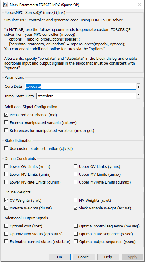
The FORCESPRO sparse QP solver is also available via the Model Predictive Control Toolbox in Simulink. A dedicated block has been implemented for this purpose. All features of the MATLAB plugin are available through this Simulink block, namely measured disturbances, external manipulated variables, references for manipulated variables,
custom state estimation as well as online weights and constraints. Configuring the block is done via the user interface shown in Figure 6.1 below. Currently only the sparse QP solver can be used via the Simulink API.
Figure 6.1 FORCESPRO LTI MPC block configuration window. FORCESPRO adaptive and LTV MPC block configuration windows have the same options available.
In order to run a simulation using the FORCESPRO Simulink block, a solver first needs to be generated via the following code for instance:
%% Generate FORCESPRO sparse QP solveroptions=mpcToForcesOptions('sparse');% If we want to use the adaptive MPC block, we need to set% options.UseAdaptive = true;% If we want to use the time-varying MPC block, we need to set% options.UseLTV = true;% For this example we need to specify that online weights on the outputs,% the input rates and the ECR slacks are usedoptions.UseOnlineWeightOV=true;options.UseOnlineWeightMVRate=true;options.UseOnlineWeightECR=true;[coredata,statedata,onlinedata]=mpcToForces(mpcobj,options);
The structures coredata and statedata needed by the FORCESPRO solver are then provided to the Simulink block via the window shown in Figure 6.1.
coredata is the variable name of the core data structure generated by mpcToForces in the base workspace.
initial state data is the variable name of the state data structure generated by mpcToForces in the base workspace. The user is expected to populate this structure with initial states of the plant and disturbances.
md checkbox should be selected if MD channels exist in the MPC object.
x[k|k] checkbox needs to be selected for using a custom state estimator.
Optional outputs provide more information. It is recommended to monitor the qp.status port to check whether the MPC block produces a feasible solution.
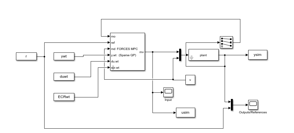
The integration of the FORCESPRO LTI MPC block in a Simulink model is shown in Figure 6.2 below.
The FORCESPRO adaptive and LTV MPC block would work equivalently with the difference that both have an additional input port for the model-struct (see Figure 6.3).
Figure 6.2 Simulink model illustrating the integration of the FORCESPRO LTI MPC block
The Simulink model can be run either by clicking on the Run button in Simulink or from MATLAB using the sim command.
% Start simulation.mdl='forcesmpc_onlinetuning';open_system(mdl);% Open Simulink(R) Modelsim(mdl);% Start Simulation
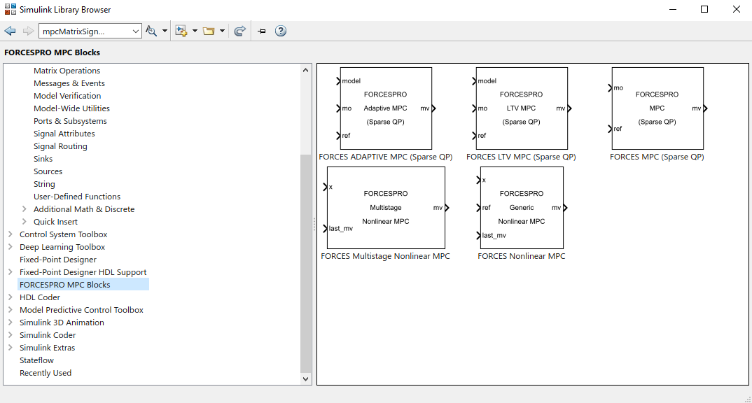
Finally, the different FORCESPRO MPC blocks (LTI/adaptive/LTV) are available via the Library browser once the user has updated his client to the latest version of FORCESPRO, as shown in Figure 6.3 below.
Figure 6.3 FORCESPRO MPC block in the library browser
FORCESPRO currently does not support the dSPACE MicroAutoBox II platform. This example has remained as a guideline for deployment to other target platforms.
The FORCESPRO sparse solvers can be used inside Simulink to deploy to dSPACE MicroAutoBox II. All features of the MATLAB plugin are available through this Simulink block, namely measured disturbances, external manipulated variables, references for manipulated variables,
custom state estimation as well as online weights and constraints. Configuring the block is done via the user interface shown in Figure 6.4 below.
In order to run an MPC simulation in dSPACE using the FORCESPRO block, a solver first needs to be generated via the following code:
%% Generate FORCESPRO sparse QP solveroptions=mpcToForcesOptions('sparse');% For this example we need to specify that online weights on the outputs,% the input rates and the ECR slacks are usedoptions.UseOnlineWeightOV=true;options.UseOnlineWeightMVRate=true;options.UseOnlineWeightECR=true;options.ForcesTargetPlatform='dSPACE-MABII';[coredata,statedata,onlinedata]=mpcToForces(mpcobj,options);
Note that the option ForcesTargetPlatform needs to be specified. The structures coredata and statedata needed by the FORCESPRO solver are then provided to the Simulink block via the window shown in Figure 6.4. The integration of the FORCESPRO MPC block in a Simulink model is shown in Figure 6.5 below.
Figure 6.5 FORCESPRO MPC block integration in a Simulink model
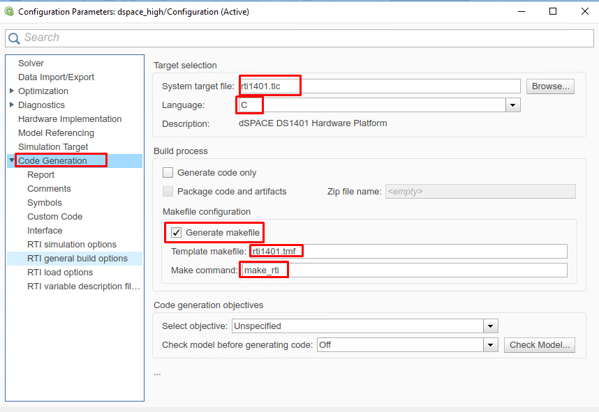
When creating the Simulink Model, in the Configurations, in the “Code Generation” tab, set the options (see Figure 6.6 below):
System target file: rti1401.tlc
Language: C
Generate makefile: On
Template makefile: rti1401.tmf
Make command: make_rti
Figure 6.6 Configure Code Generation for dSPACE MicroAutoBox II
The Simulink model can be used for Code Generation from MATLAB in the usual way.
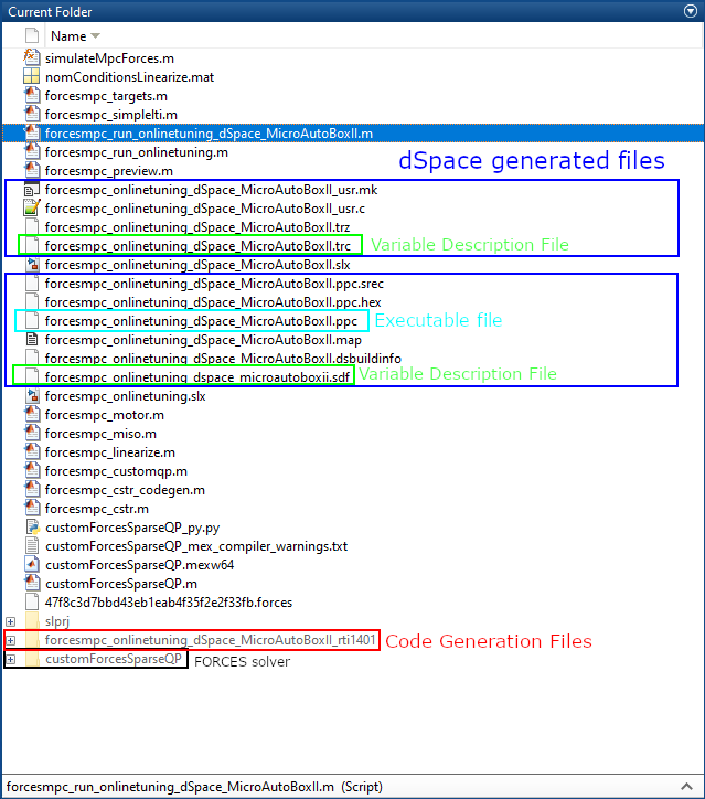
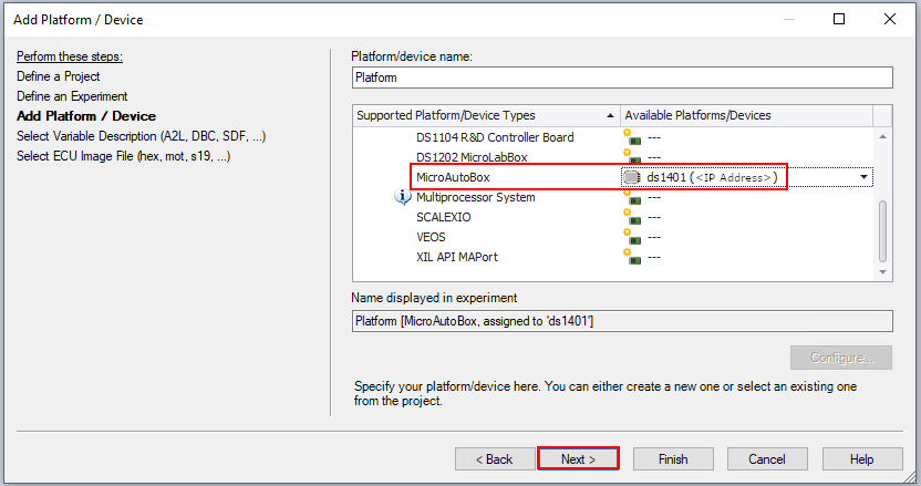
Select the platform to which you will deploy the generated executable (see Figure 6.11).
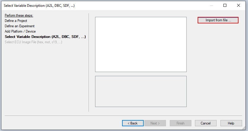
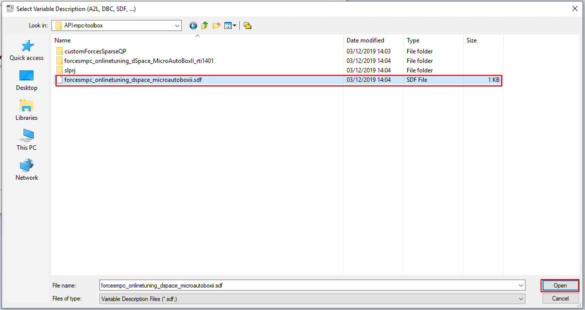
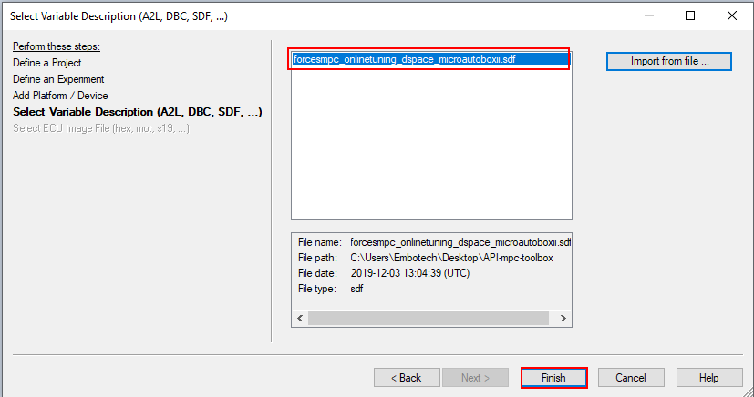
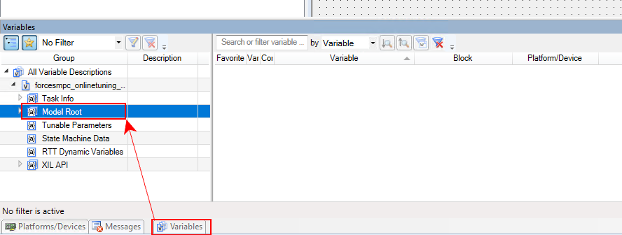
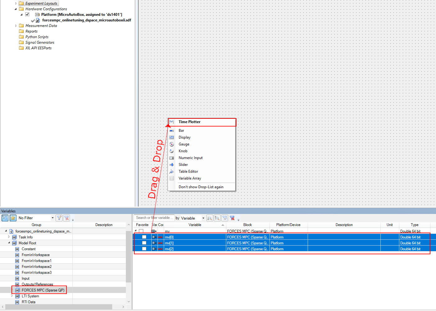
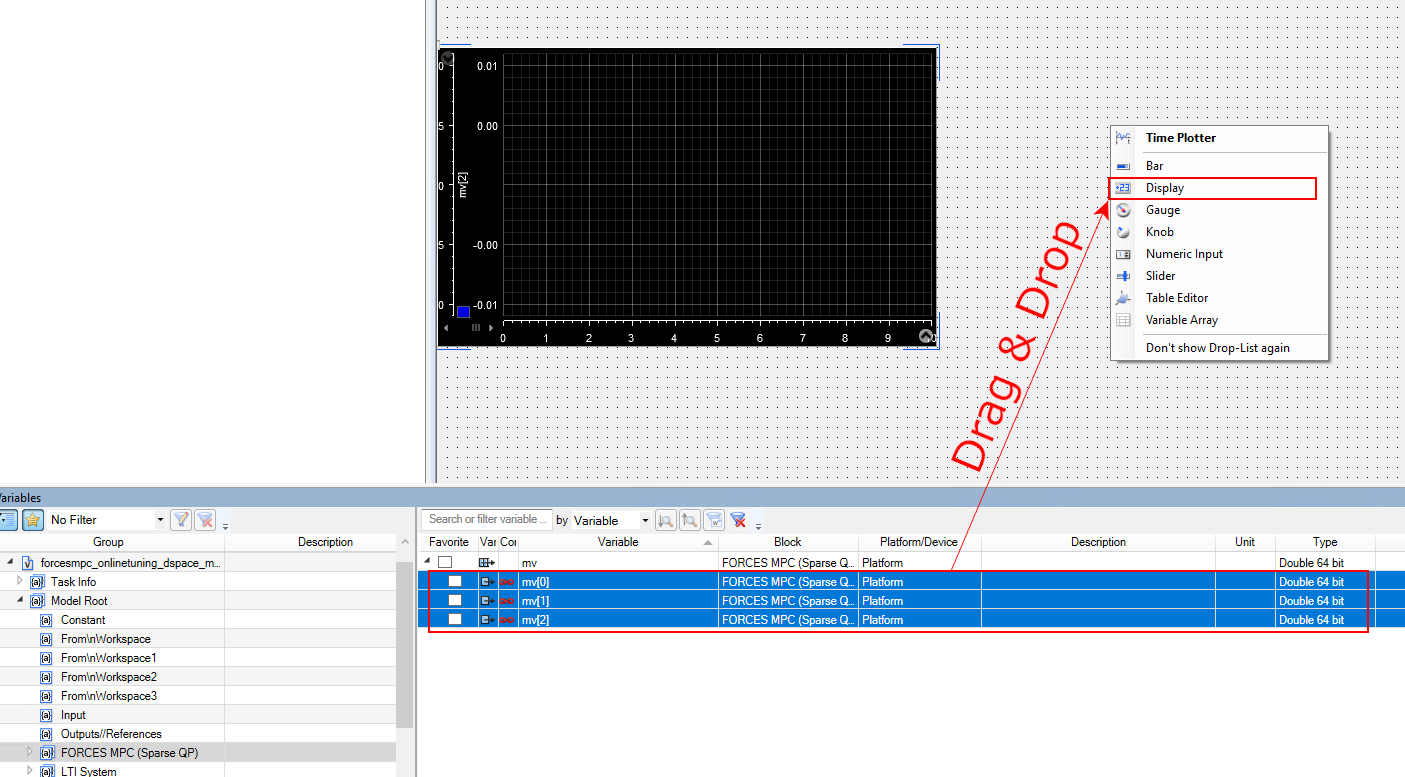
Import the variable description file forcesmpc_onlinetuning_dSpace_MicroAutoBoxII.sdf in order to have access to the model variables and see the results of the execution (see Figure 6.12 and Figure 6.13).
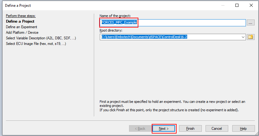
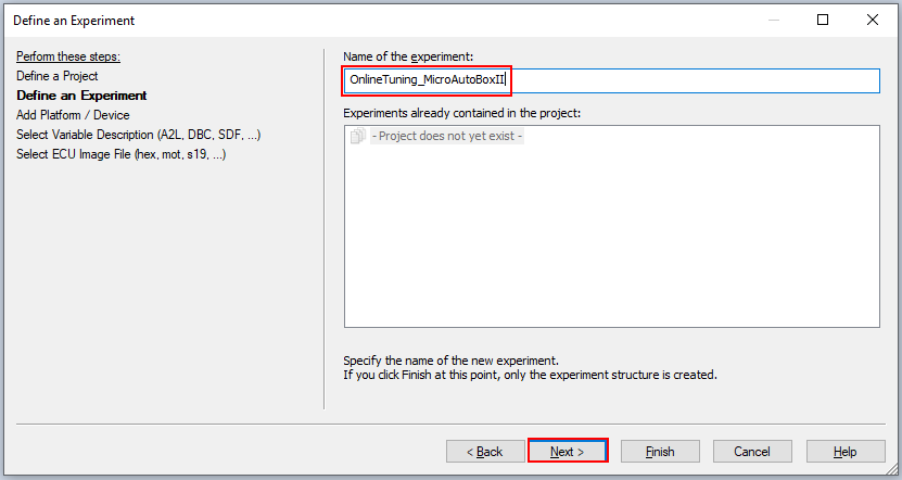
Click Finish to create the project (see Figure 6.14).
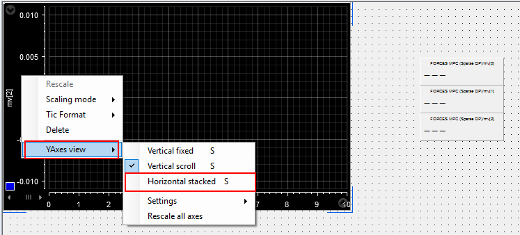
Figure 6.18 Select to show all the signals on the same plot with their own Y-axes
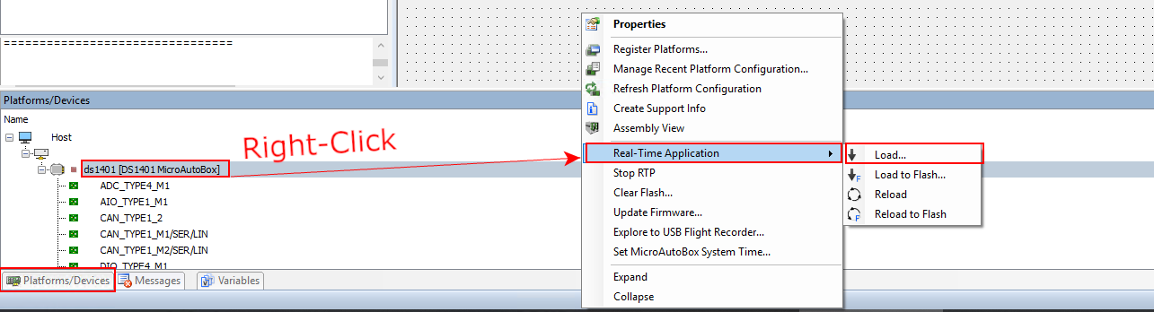
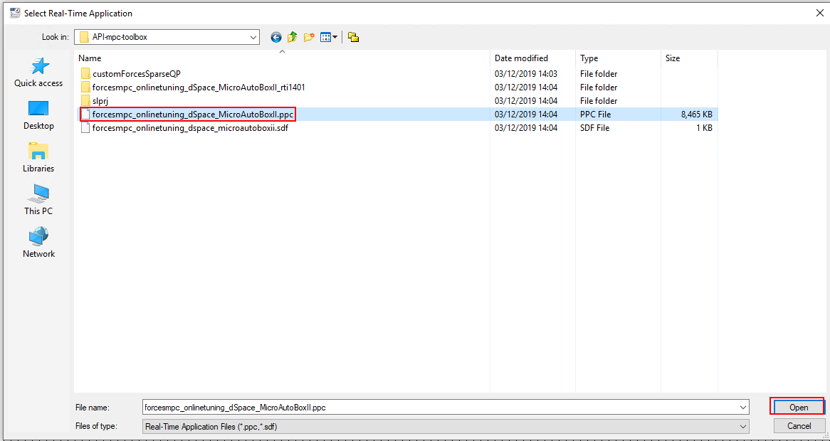
Select the Platforms/Devices tab. Right-Click on your platform and select Real-TimeApplication> Load. Choose the executable file forcesmpc_onlinetuning_dSpace_MicroAutoBoxII.ppc (see Figure 6.19 and Figure 6.20).
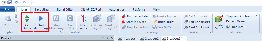
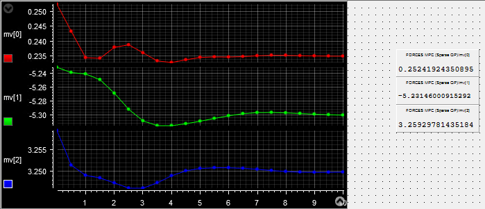
Select GoOnline and StartMeasuring to see the results. (see Figure 6.21 and Figure 6.22).
Figure 6.19 Load the application on the dSPACE MicroAutoBox II
Figure 6.20 Select the executable to run the experiment
Figure 6.21 Buttons Go Online and Start Measuring to receive execution results
Figure 6.22 Plots and results from experiment on dSPACE MicroAutoBox II
The plugin comes with several examples to demonstrate its functionalities and flexibility.
The packaged examples are the following ones:
forcesmpc_cstr.m is a linear time-invariant (LTI) MPC example with unmeasured outputs. It also shows how to use the MATLAB Coder for generating and running mpcmoveForces as a mex interface, which results in lower simulation times.
forcesmpc_timevarying.zip compares the performance of the LTI, adaptive and LTV MPC controllers, when having a time-varying plant.
In particular, it demonstrates how to use the plugin for LTI, adaptive and LTV MPC in the MATLAB environment.
In case the MATLAB Coder Toolbox is installed, it shows how to use automatically generated MEX functions for faster simulations in the MATLAB environment.
In case the Simulink Toolbox is installed, it also showcases how to run a simulation using the corresponding Simulink blocks in the Simulink environment.
The forcesmpc_linearize.m example is described in more details below. First, the linearized model and the operating point are loaded from a MAT file.
%% Load plant model linearized at its nominal operating point (x0, u0, y0)load('nomConditionsLinearize.mat');
An MPC controller object is then created with a prediction horizon of length \(p = 20\), a control horizon \(m = 3\) and a sampling period \(T_s = 0.1\) seconds as explained here.
%% Design MPC Controller% Create an MPC controller object with a specified sample time |Ts|,% prediction horizon |p|, and control horizon |m|.Ts=0.1;p=20;m=3;mpcobj=mpc(plant,Ts,p,m);
Nominal values need to be set in the MPC object.
% Set the nominal values in the controller.mpcobj.Model.Nominal=struct('X',x0,'U',u0,'Y',y0);
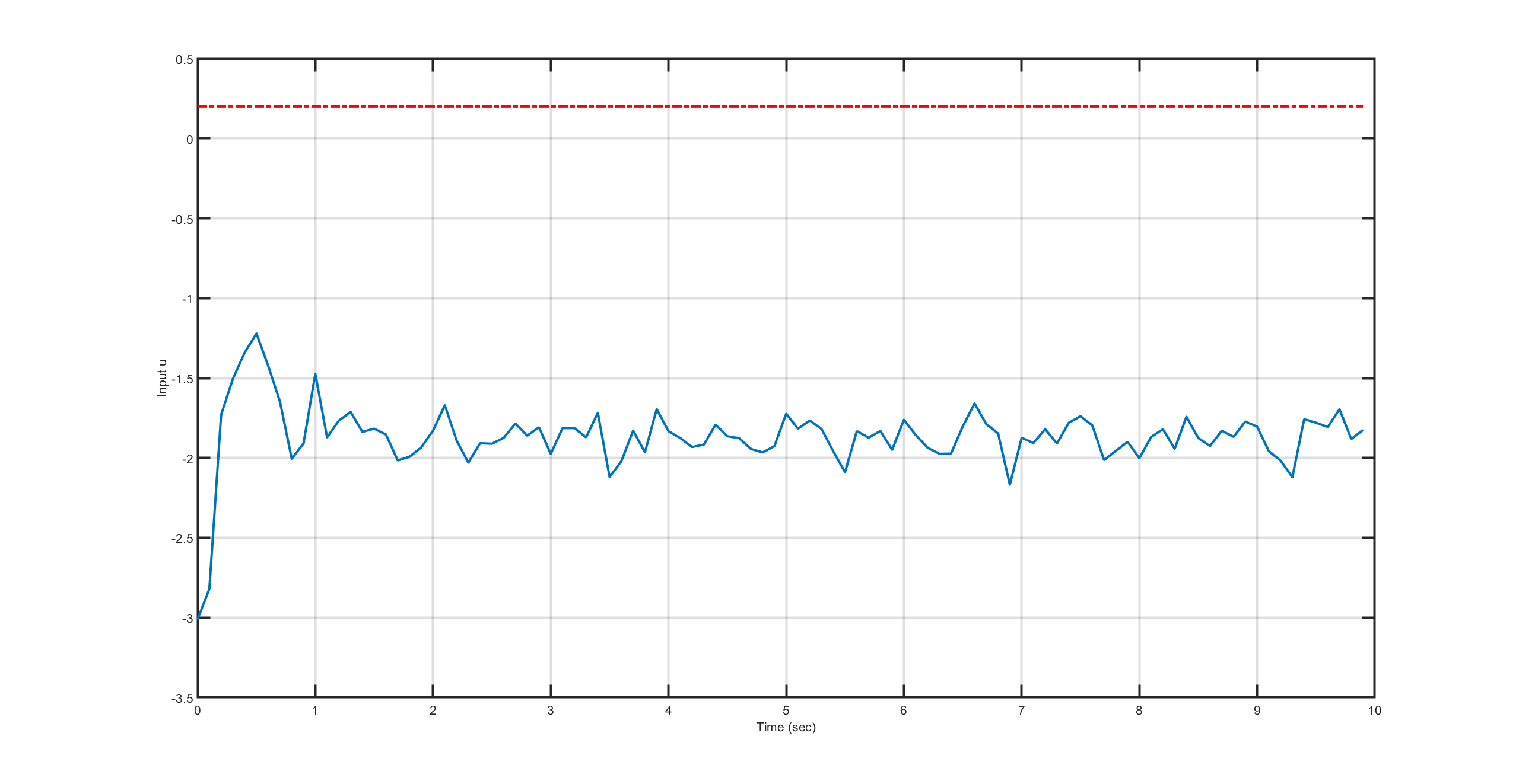
Constraints are set on the manipulated variables and an output reference signal is provided.
% Set the manipulated variable constraint.mpcobj.MV.Max=0.2;% Specify the reference value for the output signal.r0=1.5*y0;
From the MPC object and a structure of options, a FORCESPRO solver can be generated.
% Create options structure for the FORCESPRO sparse QP solveroptions=mpcToForcesOptions();% Generates the FORCESPRO QP solver[coredata,statedata,onlinedata]=mpcToForces(mpcobj,options);
Once a reference signal has been constructed, the simulation can be run using mpcmoveForces.
fort=1:Tf% A measurement noise is simulatedY(:,t)=dPlant.C*(X(:,t)-x0)+dPlant.D*(U(:,t)-u0)+y0+0.01*randn;% Prepare inputs of mpcmoveForcesonlinedata.signals.ref=r(t:min(t+mpcobj.PredictionHorizon-1,Tf),:);onlinedata.signals.ym=Y(:,t);% Call FORCESPRO solver[mv,statedata,info]=mpcmoveForces(coredata,statedata,onlinedata);ifinfo.ExitFlag<0warning('Internal problem in FORCESPRO solver');endU(:,t)=mv;X(:,t+1)=dPlant.A*(X(:,t)-x0)+dPlant.B*(U(:,t)-u0)+x0;end
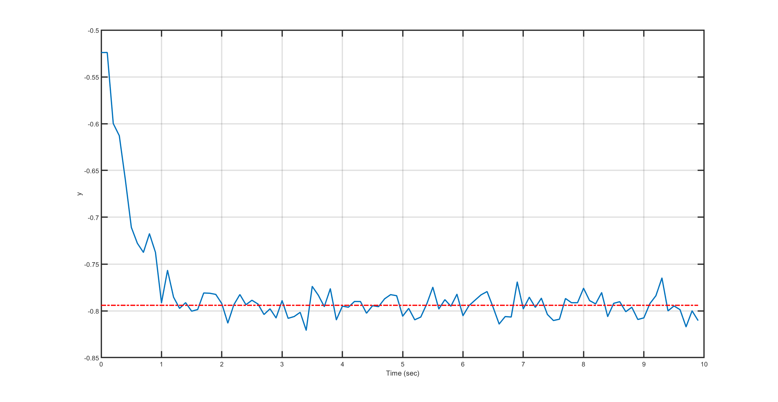
The resulting input and output signals are shown in Figure Figure 6.23 and Figure Figure 6.24 respectively.
Figure 6.23 Manipulated variable computed by the FORCESPRO plugin.
Figure 6.24 Output variable computed by the FORCESPRO plugin.
The adaptiveMPCExample.zip example is described in more details below. In particular, it showcases the difference in performance of the different linear MPC Plugin
variants, namely LTI, adaptive and LTV, when controlling a time-varying plant.
This example is an adaptation of an example from MathWorks (see here).
The time-varying model is a single-input-single-output 3rd order time-varying linear system with poles, zeros and gain that vary periodically with time.
%% Initialization% Set the simulation duration in seconds.p=3;% prediction horizonm=3;% control horizonTs=0.1;Tstop=25;Nsim=round(Tstop/Ts)+1;%% Time-Varying Plant% $$G = \frac{{5s + 5 + 2\cos \left( {2.5t} \right)}}{{{s^3}% + 3{s^2} + 2s + 6 + \sin \left( {5t} \right)}}$$%% The plant poles move between being stable and unstable at run time,% which leads to a challenging control problem.% Generate an array of plant models at |t| = |0|, |Ts|, |2*Ts|, ...,% |Tstop + p*Ts| seconds.Models=tf;ct=1;fort=0:Ts:(Tstop+p*Ts)Models(:,:,ct)=tf([55+2*cos(2.5*t)],[1326+sin(5*t)]);ct=ct+1;end% Convert the models to state-space format and discretize them with a% sample time of Ts second.Models=ss(c2d(Models,Ts));
An MPC controller object is created with a prediction and control horizon of \(p=m=3\)
and a sampling time \(T_s=0.1s\) as defined previously
%% MPC Controller Design% The control objective is to track a step change in the reference signal.% First, design an MPC controller for the average plant model. The% controller sample time is Ts second.sys=ss(c2d(tf([55],[1326]),Ts));% prediction modelmpcobj=mpc(sys,Ts,p,m);% Set hard constraints on the manipulated variable and specify tuning% weights.mpcobj.MV=struct('Min',-2,'Max',2);mpcobj.Weights=struct('MV',0,'MVRate',0.01,'Output',1);% Save relevant dimensionsnx=length(mpcobj.Model.Nominal.X);ny=length(mpcobj.Model.Nominal.Y);nu=length(mpcobj.Model.Nominal.U);% Set the initial plant states to zero.x0=zeros(nx,1);
With the MPC object and an additional options structure, the FORCESPRO solver for the LTI, adaptive and LTV case can be generated.
In case of ‘sparse’ QP formulation, if the MathWorks Toolbox MATLABCoder is installed, the mpcToForces will also generate a MEX version of mpcmoveForces and/or mpcmoveAdaptiveForces respectively.
The generated MEX function will have the name mpcmove_<options.SolverName> and/or mpcmoveAdaptive_<options.SolverName> respectively, depending on the chosen MPC variant.
We define the step reference changes to be tracked by the LTI, adaptive and LTV MPC controllers.
This references array will be used for reference previewing in all three MPC controllers.
For the LTI MPC we need to provide only the measured output and the reference preview over the prediction horizon.
If we use the MEX function, we do not need to provide the constant MATLAB structure coredataLTI.
%% SimulationcoderIsInstalled=mpcchecktoolboxinstalled('matlabcoder');% LTIyyMPCFORCES=zeros(ny,Nsim);uuMPCFORCES=zeros(nu,Nsim);x=x0;forct=1:Nsim% Get the real plant.real_plant=Models(:,:,ct);% Update and store the plant output.y=real_plant.C*x;yyMPCFORCES(ct)=y;% Compute and store the MPC optimal move.onlinedataLTI.signals.ym=y;onlinedataLTI.signals.ref=references(ct:ct+p-1);ifcoderIsInstalled% MEX function name is mpcmove_<optionsLTI.SolverName>% It is not necessary to supply the constant coredataLTI (i.e.% it was already considered during code generation)[mv,statedataLTI,~]=mpcmove_LTICustomForcesSparseQP(statedataLTI,onlinedataLTI);else[mv,statedataLTI,~]=mpcmoveForces(coredataLTI,statedataLTI,onlinedataLTI);enduuMPCFORCES(ct)=mv;% Update the plant state.x=real_plant.A*x+real_plant.B*mv;end
For the adaptive MPC we can provide the plant matrices and the nominals at the current timestep in addition to the measured output and the reference preview over the prediction horizon.
If we use the MEX function, we do not need to provide the constant MATLAB structure coredataAdaptive.
% AdaptiveyyAMPCFORCES=zeros(ny,Nsim);uuAMPCFORCES=zeros(nu,Nsim);x=x0;nominal=mpcobj.Model.Nominal;% Nominal conditions are constant over the prediction horizon.forct=1:Nsim% Get the real plant.real_plant=Models(:,:,ct);% Update and store the plant output.y=real_plant.C*x;yyAMPCFORCES(ct)=y;% Compute and store the MPC optimal move.onlinedataAdaptive.signals.ym=y;onlinedataAdaptive.signals.ref=references(ct:ct+p-1);onlinedataAdaptive.model.X=nominal.X;onlinedataAdaptive.model.U=nominal.U;onlinedataAdaptive.model.Y=nominal.Y;onlinedataAdaptive.model.DX=nominal.DX;onlinedataAdaptive.model.A=real_plant.A;onlinedataAdaptive.model.B=real_plant.B;onlinedataAdaptive.model.C=real_plant.C;onlinedataAdaptive.model.D=real_plant.D;ifcoderIsInstalled% MEX function name is mpcmoveAdaptive_<optionsAdaptive.SolverName>% It is not necessary to supply the constant coredataAdaptive% (i.e. it was already considered during code generation)[mv,statedataAdaptive,~]=mpcmoveAdaptive_AdaptiveCustomForcesSparseQP(statedataAdaptive,onlinedataAdaptive);else[mv,statedataAdaptive,~]=mpcmoveAdaptiveForces(coredataAdaptive,statedataAdaptive,onlinedataAdaptive);enduuAMPCFORCES(ct)=mv;% Update the plant state.x=real_plant.A*x+real_plant.B*mv;end
For the LTV MPC we can provide the plant matrices and the nominals over the prediction horizon in addition to the measured output and the reference preview over the prediction horizon.
If we use the MEX function, we do not need to provide the constant MATLAB structure coredataLTV.
% LTVyyLTVMPCFORCES=zeros(ny,Nsim);uuLTVMPCFORCES=zeros(nu,Nsim);x=x0;Nominals=repmat(mpcobj.Model.Nominal,p+1,1);% Nominal conditions are constant over the prediction horizon.forct=1:Nsim% Get the real plant.real_plant=Models(:,:,ct);% Update and store the plant output.y=real_plant.C*x;yyLTVMPCFORCES(ct)=y;% Compute and store the MPC optimal move.onlinedataLTV.signals.ym=y;onlinedataLTV.signals.ref=references(ct:ct+p-1);fork=1:p+1onlinedataLTV.model.X(:,1,k)=Nominals(k).X;onlinedataLTV.model.DX(:,1,k)=Nominals(k).DX;onlinedataLTV.model.U(:,1,k)=Nominals(k).U;onlinedataLTV.model.Y(:,1,k)=Nominals(k).Y;model=Models(:,:,ct+k-1);onlinedataLTV.model.A(:,:,k)=model.A;onlinedataLTV.model.B(:,:,k)=model.B;onlinedataLTV.model.C(:,:,k)=model.C;onlinedataLTV.model.D(:,:,k)=model.D;endifcoderIsInstalled% MEX function name is mpcmoveAdaptive_<optionsLTV.SolverName>% It is not necessary to supply the constant coredataLTV (i.e.% it was already considered during code generation)[mv,statedataLTV,~]=mpcmoveAdaptive_LTVCustomForcesSparseQP(statedataLTV,onlinedataLTV);else[mv,statedataLTV,~]=mpcmoveAdaptiveForces(coredataLTV,statedataLTV,onlinedataLTV);enduuLTVMPCFORCES(ct)=mv;% Update the plant state.x=real_plant.A*x+real_plant.B*mv;end
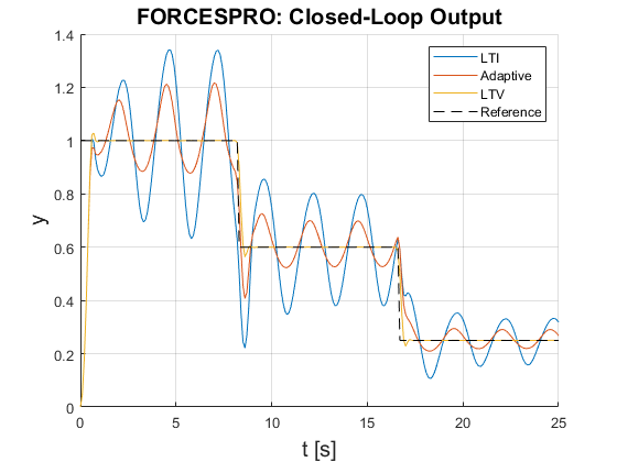
The resulting control performance of all three MPC variants are shown in Figure Figure 6.25.
We can see that the LTI has big oscillatory deviations from the references.
Using the adaptive MPC, which changes the model in each timestep while keeping it constant over the prediction horizon, improves performance
resulting in smaller deviations from the references.
By using the LTV MPC, the user can provide specific models for each of the p+1 stages of the prediction horizon in each timestep, so that
the tracking performance becomes almost flawless with minimal deviations only.
Figure 6.25 Output variable tracking performance for LTI, adaptive and LTV MPC variants.
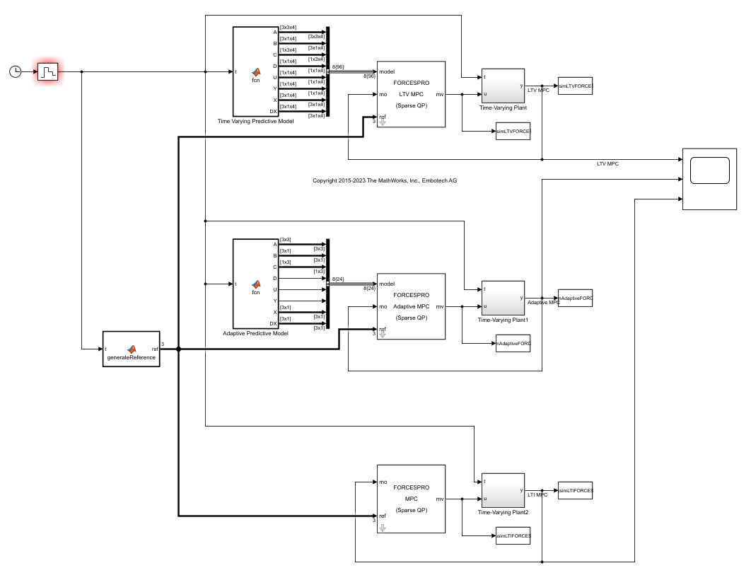
In the provided example scripts, we additionally show how to run the closed-loop simulation for LTI, adaptive and LTV MPC controllers in the Simulink environment. The corresponding Simulink model looks like Figure Figure 6.26
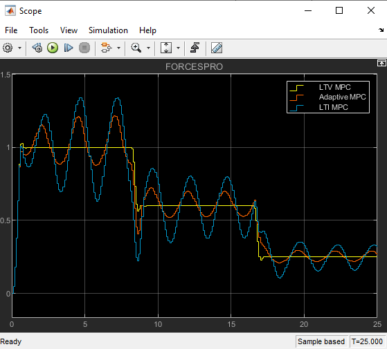
and the corresponding results (see Figure Figure 6.27) match with the results from the MATLAB environment (see Figure Figure 6.25).
Figure 6.26 Simulink model of closed-loop simulation for a time-varying plant using LTI, adaptive and LTV MPC controllers
Figure 6.27 Scope plot of the Simulink closed-loop simulation result of Figure Figure 6.26