11.16. Real-time SQP Solver: Robotic Arm Manipulator (MATLAB & Python)

In this example we illustrate the use of the real-time Sequential Quadratic Programming (SQP) solver and how to generate and call the dynamics used in the formulation of the optimization problem directly in MATLAB/Python. In particular, we use a robotic arm manipulator described by a set of ordinary differential equations (ODEs):

\[\begin{split}\ddot{\theta}_1 =~& \gamma \\ \ddot{\theta}_2 =~& \frac{1}{\beta_2}(\tau_2 - \beta_1\gamma - \beta_3\dot{\theta}_1^2 - \beta_4) \\ \dot{\tau}_1 =~& u_1 \\ \dot{\tau}_2 =~& u_2\end{split}\]

where \(\theta_1, \theta_2\) are joint angles modelling the manipulator configuration, \(u_1, u_2\) are the rates (inputs) of the torques \(\tau_1, \tau_2\) applied to the joints and

\[\gamma~\hat{=}~\frac{1}{\alpha_1 - \alpha_2 \frac{\beta_1}{\beta_2}}(\frac{\alpha_2}{\beta_2}(\beta_4 + \beta_3\dot{\theta}_1^2 - \tau_2) - \alpha_3\dot{\theta}_1\dot{\theta}_2 - \alpha_4\dot{\theta}_2 - \alpha_5 + \tau_1).\]

The coefficients \(\alpha_1, \alpha_2, \alpha_3, \alpha_4, \alpha_5\) and \(\beta_1, \beta_2, \beta_3, \beta_4\) depend on the inertia and mass of the robot arm components. Their expressions can be found in [SicSci09]. The optimal control problem is formalized from the state \(x\) defined by

\[x~\hat{=}~(\theta_1, \dot{\theta}_1, \theta_2, \dot{\theta}_2, \tau_1, \tau_2)^{\top}\]

and the input \(u\) defined as

\[u~\hat{=}~(\dot{\tau}_1, \dot{\tau}_2)^{\top}.\]

The control objective is to make the first joint angle \(\theta_1\) follow a reference of \(1.2\,\mathrm{rad}\) from \(0\) to \(10\,\mathrm{s}\) and \(-1.2\,\mathrm{rad}\) from \(10\) to \(20\,\mathrm{s}\). Similarly, the second joint angle \(\theta_2\) should follow a reference of \(-1.2\,\mathrm{rad}\) from \(0\) to \(10\,\mathrm{s}\) and \(1.2\,\mathrm{rad}\) from \(10\) to \(20\,\mathrm{s}\). The stage variable \(z\) is defined by stacking the input and differential state variables:

\[z = (\dot{\tau}_1, \dot{\tau}_2, \theta_1, \dot{\theta}_1, \theta_2, \dot{\theta}_2, \tau_1, \tau_2)^\top\]

You can download the MATLAB code of this example to try it out for yourself by clicking here along with the dynamics here. The Python code is available here along with the dynamics here.

11.16.1. Defining the MPC problem

11.16.1.1. Tracking objective

Our goal is to minimize the distance of the joint angles to the reference, which can be translated in the following stage cost function:

\[f(z,p) = 1000(z_3 - 1.2p)^2 + 0.1z_4^2 + 1000(z_5 + 1.2p)^2 + 0.1z_6^2 + 0.01z_7^2 + 0.01z_8^2 + 0.01z_1^2 + 0.01z_2^2,\]

where \(p\) is a run-time parameter taking value \(1\) from \(0\) to \(10\,\mathrm{s}\) and \(-1\) from \(10\) to \(20\,\mathrm{s}\).

The stage cost function is coded in MATLAB as the least-squares vector:

MatlabPython

model.LSobjective = @(z,p)[sqrt(1000) * (z(3)-p(1)*1.2);...
                           sqrt(0.1) * z(4);...
                           sqrt(1000) * (z(5)+p(1)*1.2);...
                           sqrt(0.1) * z(6);...
                           sqrt(0.01) * z(7);...
                           sqrt(0.01) * z(8);...
                           sqrt(0.01) * z(1);...
                           sqrt(0.01) * z(2)];

In the MATLAB example, this is needed to compute a Gauss-Newton approximation from the Jacobian of the least-squares vector. In the Python example, where Gauss-Newton approximations are not yet available, we use the objective field to supply the target function.

11.16.1.2. State and input constraints

The following constraints are imposed on the torques and torque rates:

\begin{align*} -100\,\mathrm{Nm}\leq & \tau_1 \leq 70\,\mathrm{Nm} \\ -100\,\mathrm{Nm}\leq & \tau_2 \leq 70\,\mathrm{Nm} \\ -200\,\mathrm{Nm/s}\leq & \dot{\tau}_1 \leq 200\,\mathrm{Nm/s} \\ -200\,\mathrm{Nm/s}\leq & \dot{\tau}_2 \leq 200\,\mathrm{Nm/s} \\ \end{align*}

This corresponds to the code below.

MatlabPython

% upper/lower variable bounds lb <= x <= ub
model.lb = [ -200, -200,  -pi, -100,  -pi, -100, -100, -100 ];
model.ub = [  200,  200,   pi,  100,   pi,  100,   70,   70 ];

11.16.1.3. Initial condition and horizon length

The prediction horizon is set to \(21\) and the following initial condition is set

MatlabPython

model.xinit = [-0.4 0 0.4 0 0 0 ]';
model.xinitidx = 3:8;

11.16.2. Generating a real-time SQP solver

We have now populated model with the necessary fields to generate an SQP solver, which requires settings a few options, as follows:

MatlabPython

%% Define solver options
codeoptions = getOptions('RobotArmSolver');
codeoptions.maxit = 200;                                    % Maximum number of iterations of inner QP solver
codeoptions.printlevel = 0;                                 % Use printlevel = 2 to print progress (but not for timing)
codeoptions.optlevel = 3;
% Explicit Runge-Kutta 4 integrator
codeoptions.nlp.integrator.Ts = integrator_stepsize;
codeoptions.nlp.integrator.nodes = 5;
codeoptions.nlp.integrator.type = 'ERK4';
% Options for SQP solver
codeoptions.solvemethod = 'SQP_NLP';                        % SQP algorithm
codeoptions.nlp.hessian_approximation = 'gauss-newton';     % Gauss-Newton hessian approximation of nonlinear least-squares objective
codeoptions.sqp_nlp.use_line_search = 0;                    % Disable line-search for efficiency (only doable with Gauss-Newton approximation)
codeoptions.MEXinterface.dynamics = 1;                      % generate MEX entry point for the dynamics used in the model

%% Generate real-time SQP solver
FORCES_NLP(model, codeoptions);

The number of solved QPs in every iteration is set via sqp_nlp.maxSQPit. It is important to note that disabling the line search in the SQP algorithm does not guarantee global convergence and hence may result in less robust performance, but produces much faster solve times. Turning off the line search via sqp_nlp.use_line_search is only allowed when the Gauss-Newton approximation is on.

11.16.3. Calling the generated SQP solver

Once all parameters have been populated, the MEX interface of the solver can be used to invoke it from MATLAB, or the Python Solver class can be used to use it from within Python:

MatlabPython

% Set primal initial guess
x0i = model.lb+(model.ub-model.lb)/2;
x0 = repmat(x0i',model.N,1);
problem.x0 = x0;

% Set reference as run-time parameter
problem.all_parameters = ones(model.N,1);

% Set initial condition
problem.xinit = X(:,i);

% Call SQP solver
[output, exitflag, info] = RobotArmSolver(problem);

The RobotArmSolver is expected to return an exitflag equal to \(1\), which corresponds to a successful solver. However, note that the QP could become infeasible in some cases. In this case, one should expect an exitflag of \(-8\).

11.16.4. Calling the dynamics used in the model directly in MATLAB/Python

The MEX interface for the dynamics used in the formulation of the optimization problem can also be called directly in MATLAB and in Python, the Solver class has a method which can compute the dynamics along with its derivative (see section Calling the nonlinear functions from MATLAB or Python). This is convenient for debugging a solver formulation or simulating the system dynamics. This can be done as follows:

MatlabPython

% Set data at first stage
z = problem.x0(1:model.nvar);
p = problem.all_parameters(1:model.npar);

[c, jacc] = RobotArmSolver_dynamics(z, p);

This stores the integrated stage in c and its jacobian with respect to z in jacc.

11.16.5. Results

The control objective is to track the joint references of \(-1.2\,\mathrm{rad}\) and \(1.2\,\mathrm{rad}\) respectively, while keeping the input torque rates below \(200\,\mathrm{Nm/s}\) in magnitude and the torque states between \(-100\,\mathrm{N}\) and \(70\,\mathrm{Nm}\).

The joint angle and torques trajectories are shown in Figure Figure 11.49 and Figure Figure 11.50 respectively, while the input torque rates are plotted in Figure Figure 11.51. The closed-loop objective, which is a measure of the control performance is shown in Figure Figure 11.52.

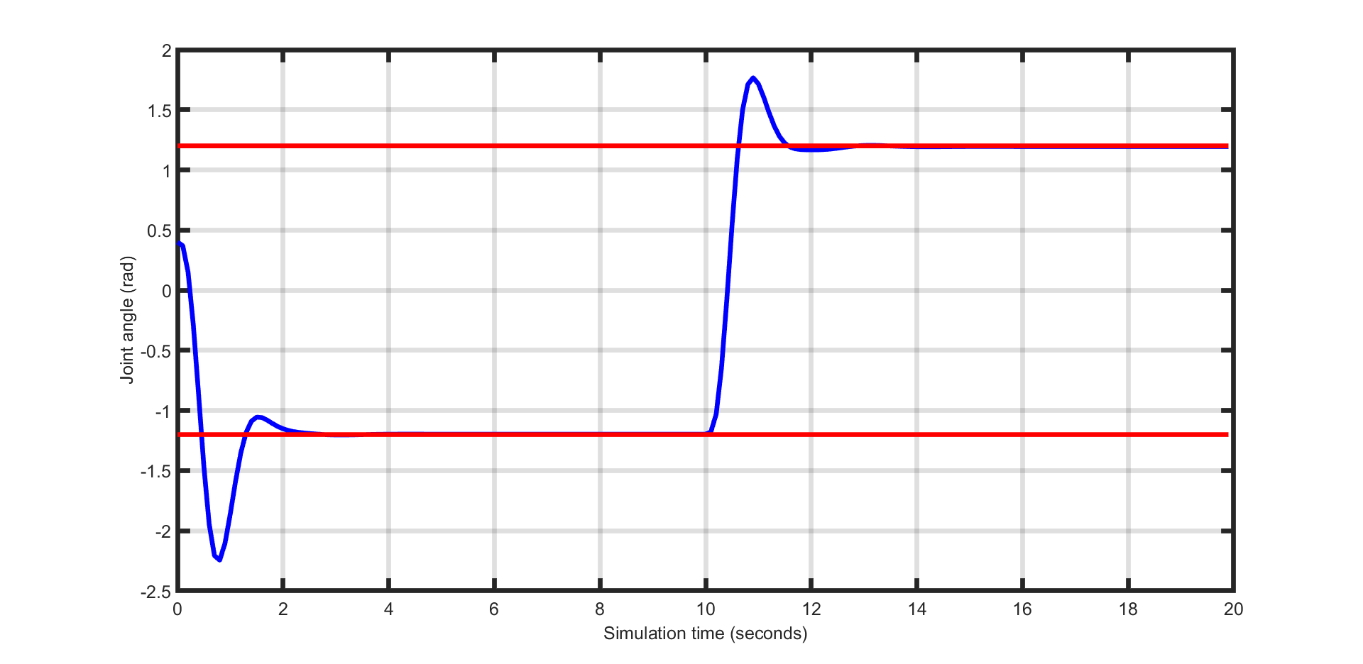
Figure 11.49 Manipulator’s joint angle.

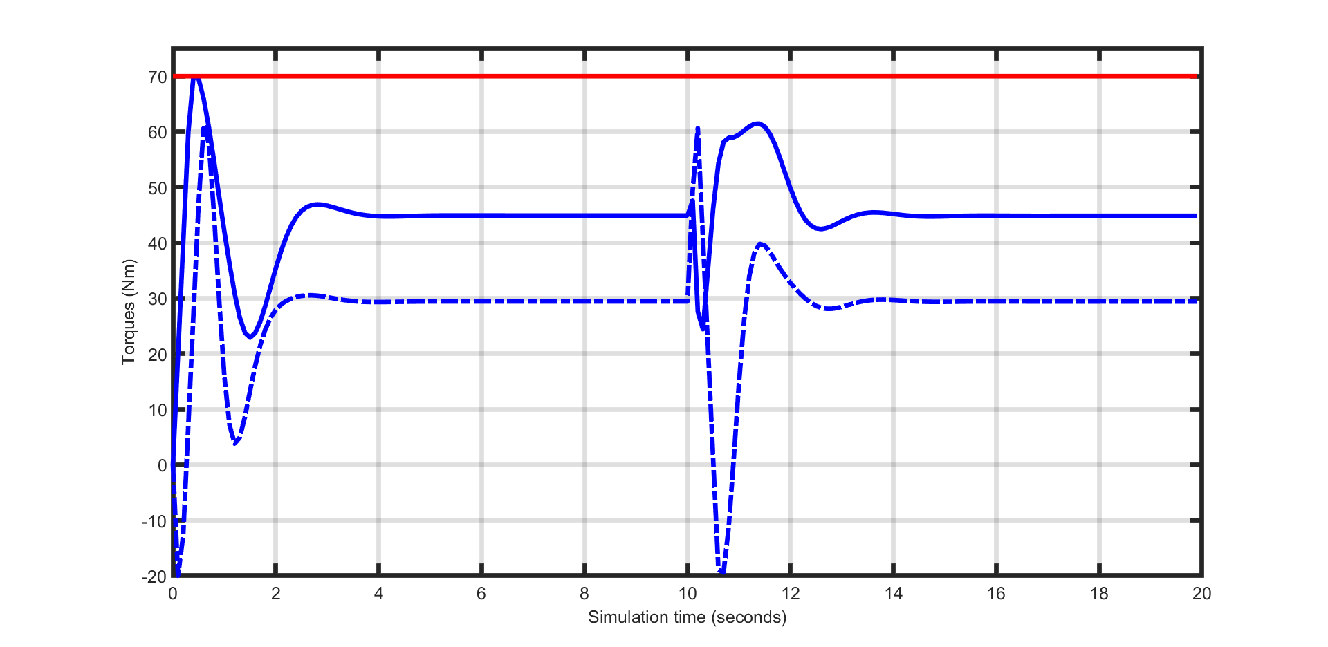
Figure 11.50 Manipulator’s torques at joints.

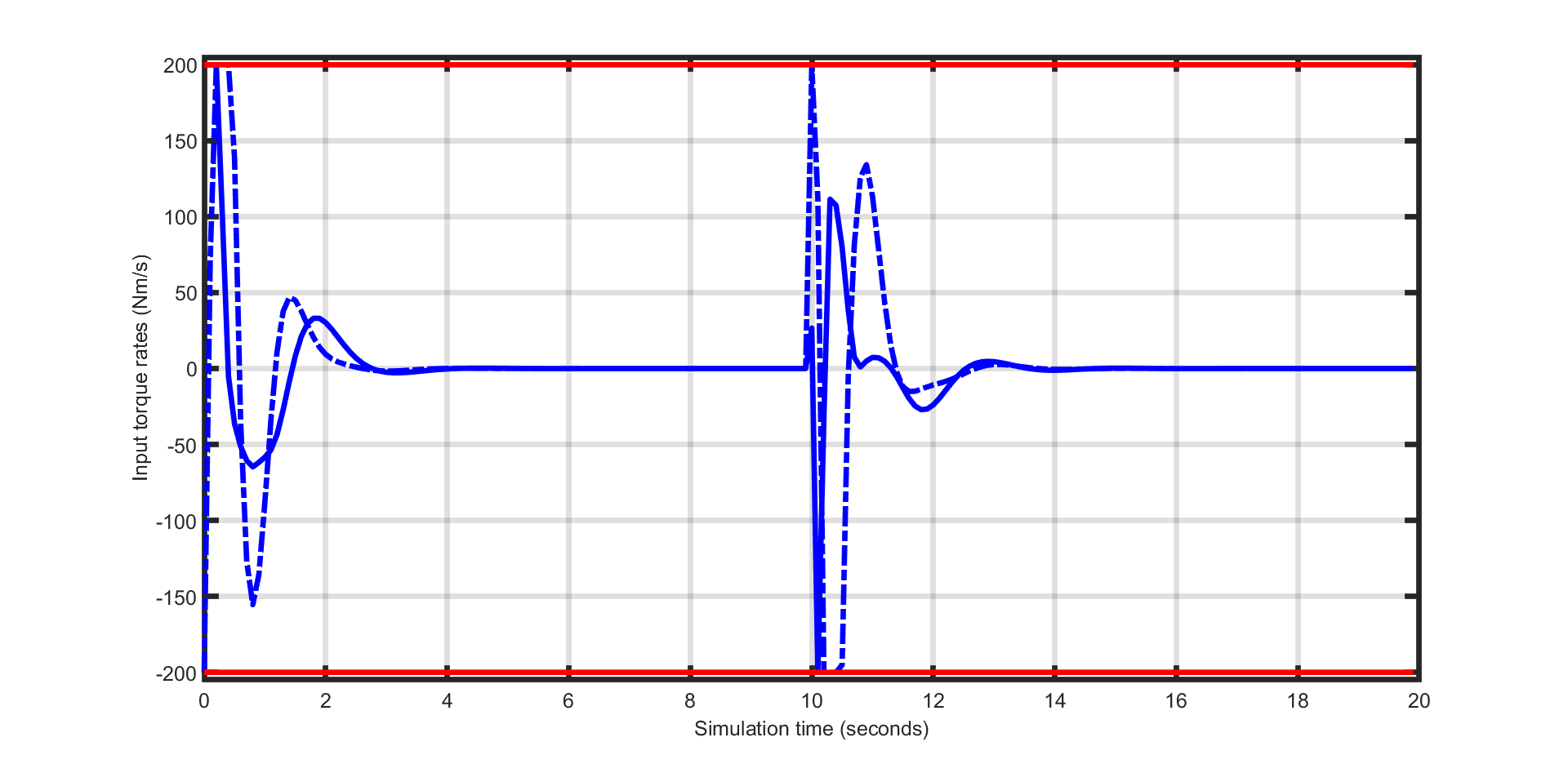
Figure 11.51 Manipulator’s torque rates.

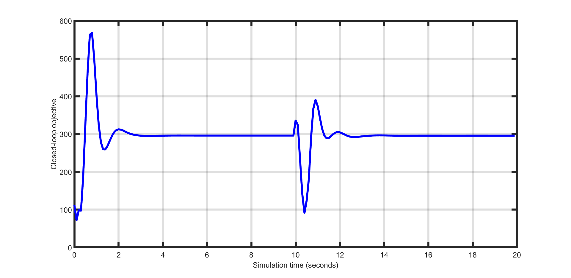
Figure 11.52 Manipulator’s closed loop objective.

[SicSci09]

Siciliano, B.; Sciavicco, L.; Villani, L.; Oriolo, G.. Robotics: Modelling, planning and control. Berlin: Springer, 2009.