7. MathWorks Nonlinear MPC Plugin¶

7.1. Introduction ¶

As a result of a long-term collaboration, MathWorks Inc. and embotech AG have extended the Model Predictive Control Toolbox™ with a plugin for the FORCESPRO nonlinear solvers. Users are now able to use the FORCESPRO nonlinear interior-point (IP) and sequential quadratic programming (SQP) solvers in MATLAB® and Simulink® from within the MATLAB® Model Predictive Control Toolbox within the nonlinear MPC API. This plugin leverages the powerful design capabilities of the Model Predictive Control Toolbox™ and the computational performance of FORCESPRO. FORCESPRO extends the Model Predictive Control Toolbox with code-generated IP and SQP solvers that are not based on finite-difference derivatives computation, resulting in faster convergence. Thanks to FORCESPRO, the nonlinear API now comes with two classes of nonlinear solvers compatible with code generation that can be deployed to various real-time targets.

Generating a FORCESPRO solver through the Model Predictive Control Toolbox plugin is done by first generating either a nlmpcMultistage object (see here) or a nlmpc object (see here). The nlmpcMultistage formulation of a nonlinear MPC problem offers maximum flexibility and customizability while also ensures optimal performance. Meanwhile, the nlmpc formulation of a nonlinear MPC problem is very easy and requires a minimal amount of coding to get started. The different aspects of generating these different objects will be covered in details below.

Depending on the object chosen, the FORCESPRO nonlinear MPC plugin consists of two API methods:

nlmpc
- nlmpcToForces generates a FORCESPRO nonlinear solver from a nonlinear MPC (nlmpc) object designed by the Model Predictive Control Toolbox
- nlmpcmoveForces calls the generated solver to calculate optimal control actions
nlmpcMultistage
- nlmpcMultistageToForces generates a FORCESPRO nonlinear solver from a nonlinear MPC multistage (nlmpcMultistage) object designed by the Model Predictive Control Toolbox
- nlmpcmoveForcesMultistage calls the generated solver to calculate optimal control actions

The nonlinear plugin also comes with Simulink® libraries that enable users to run the FORCESPRO solvers from within their Simulink® models. The generation of FORCESPRO nonlinear solvers from nlmpc objects is supported from MATLAB R2020a while generation from nlmpcMultistage objects is supported from MATLAB R2021a.

This interface is provided with Variant L and partially with Variant M of FORCESPRO.

Important

Note that when generating a FORCESPRO solver using a nlmpcMultistage object there is the following caveat concerning declaration of model functions: For any stage cost, equality and inequality constraint function, if it is defined differently than any other stage, it must be specified in a separate MATLAB function. In other words, do not define different cost and constraint terms in a single function using a switch yard based on stage number. Instead, use different functions, one for each unique definition.

For example, do not use a single cost function and assign it to every stage like showed in the following code-snippet:

% THIS WILL NOT WORK CORRECTLY!
function cost = LaneFollowingCostFcn(stage,x,u,dmv,para)
Wx = [0; 0; 0.05; 0; 3; 0];
Wdmv = [0.1; 0.2];
ref = [0; 0; para(2); 0; 0; 0];
p = para(1)
if stage==1
cost = (Wdmv.*dmv)'*(Wdmv.*dmv);
elseif stage==(p+1)
  cost = (Wx.*(x-ref))'*(Wx.*(x-ref));
else
  cost = (Wx.*(x-ref))'*(Wx.*(x-ref)) + (Wdmv.*dmv)'*(Wdmv.*dmv);
end

Instead, split it into three functions and assign them to $1$, $2$ to $p$ and $p+1$ respectively.

7.2. The SQP Fast algorithm for nlmpc ¶

From FORCESPRO version 6.0.0, in addition to the previously supported interior point and general SQP algorithms, a new SQP Fast algorithm was added. The workflow for the SQP Fast algorithm is slightly different from the workflow required to generate solvers using the other algorithms. The main difference is that generating a SQP Fast solver required a tuning step. The core idea behind this is that it allows for a highly specialized/tailored SQP algorithm which achieves optimal performance for a given MPC application. For this purpose FORCESPRO ships a caching tool for collecting simulation data in order to tune the SQP Fast solver. The generation of a SQP Fast solver is controlled via the caching tool. The caching tool is a simple mechanism and interacting with it goes via three commands:

forcesMpcCache clear: Deletes all stored caches completely.
forcesMpCache on: Turns on the cache by constructing a cache object. This command must be called before nlmpcToForces is called in order to properly cache simulation data. From when the cache is turned on until it is turned off, every call to the generated solver via nlmpcmoveForces will store a problem instance in the cache, so it can later be used for tuning the SQP Fast solver.
forcesMpcCache off: Stores the allocated cache in a folder named “FORCESPRO_CACHE” and deletes the cache object from the base workspace.
forcesMpcCache reset: Equivalent to forcesMpcCache clear; forcesMpcCache on.

When no cache has been stored (default) a SQP General solver is generated when calling nlmpcToForces. If on the other hand a cache is available when calling nlmpcToForces, then a SQP Fast solver is generated. Hence, after constructing and specifying an NLMPC object nlmpcobj, the complete workflow for generating a SQP Fast solver is as follows:

Turn on the FORCESPRO cache by running forcesMpcCache on (or forcesMpcCache reset) in the MATLAB terminal.
Generate a SQP General solver by calling nlmpcToForces(nlmpcobj,options) with options.SolverType = 'SQP' (see Using an “nlmpc” object).
Run a simulation, using nlmpcmoveForces to compute optimal control moves. It is important that nlmpcmoveForces is used as opposed to the generated MEX file, which is not able to cache the problem data for tuning the fast SQP solver.
Turn off the cache by running forcesMpcCache off in the MATLAB terminal.
Generate a QP fast solver by calling nlmpcToForces(nlmpcobj,options) (see Using an “nlmpc” object). Since the cache has been stored in step 4, a SQP Fast solver will be generated and the automatic tuning procedure will be triggered.

See an example here where the full workflow is described in full detail.

Important

If the MATLAB command clear is called in between the calls forcesMpcCache on and forcesMpcCache off the cache is deleted. Hence, this should be avoided.

Important

The SQP Fast solver is currently only supported when generating a solver using a nlmpc object (see Using an “nlmpc” object).

7.3. Defining a nonlinear model ¶

In order to call the FORCESPRO code generation, both a nlmpc object as well as a nlmpcMultistage object need to be built from a Model. The process is essentially the same as the one described here. However one should note that the FORCESPRO code generation ignores the jacobian functions that may be provided in Jacobian.StateFcn and Jacobian.OutputFcn, since these will be automatically generated by the automatic differentiation tool CasADi. Moreover, the following requirements on the fields Model.StateFcn and Model.OutputFcn need to be fulfilled for the plugin to work seamlessly:

they must be the name of a function file, not an anonymous functions

they must be compatible with MATLAB code generation

they must follow CasADi coding conventions. Most importantly, the state derivative dxdt has to be built explicitly, as shown below.
dxdt = [expression; expression; …]

As a word of caution, the following code snippet will result in an undesired behavior from CasADI.

dxdt = x;            % Do not write this, CasADI takes it as reference !
dxdt(1,1) = a1*x(1) + a2*x(2) + b1*u(2);
dxdt(2,1) = a3*x(1) + a4*x(2) + b2*u(2);
dxdt(3,1) = x(2)*x(1) + x(4);
dxdt(4,1) = (1/tau)*(-x(4) + u(1));
dxdt(5,1) = x(1) + x(3)*x(6);
dxdt(6,1) = x(2) - 0*x(3);

FORCESPRO calls the model functions from its own objects, which follow an assignment by reference convention, hence the assignment dxdt = x is made by reference. This implies that updating dxdt also changes x, which builds the wrong symbolic dynamics.

For nlmpc objects, if the model contains a parameter, it must be a single vector parameter. In other words, users need to set nlobj.Model.NumberOfParameters = 1 and at run-time write onlinedata.Parameter = value where value is a column vector.

7.4. Generating an NLP solver ¶

7.4.1. Using an “nlmpc” object ¶

When generating a FORCESPRO solver using an nlmpc object, the main difference compared to the existing nonlinear MPC from The MathWorks based on the fmincon solver from the Optimization Toolbox is a code generation step that takes the nonlinear MPC object as argument. This is needed in order to build a mex interface for a FORCESPRO nonlinear solver that is customized to the model provided by the user.

Given an NLMPC object created by the nlmpc command, users can generate an IP or SQP nonlinear solver tailored to their specific problem via the following command:

% nlobj is the output of nlmpc(...)
% options is the output of nlmpcToForcesOptions(...)

[coredata, onlinedata] = nlmpcToForces(nlobj, options);

Two types of nonlinear solvers can be generated via nlmpcToForces: a nonlinear interior-point solver and a sequential quadratic programming solver whose features are covered in details in Sequential quadratic programming algorithm.

The nlmpcToForces API is described in more details in the tables below. The nlmpcToForces command expects an NLMPC object nlobj and a structure options as arguments. It also has a few limitations as it currently does not support custom cost and constraints. Instead one should in this case use an nlmpcMultistage object to represent custom cost and constraints. It also requires double precision.

Table 7.1 nlmpcToForces arguments¶
Input	Description
nlobj	NMPC object constructed by Model Predictive Control Toolbox (see here)
options	Object that provides solver generation options.

The outputs of nlmpcToForces consist of two structures coredata, a structure containing the constant NLMPC information used by nlmpcmoveForces and onlinedata, a structure that allows you to specify online signals such as x, lastMV, ref, MVTarget, md as well as weights or bounds used by nlmpcmoveForces.

In order to provide the solver options to nlmpcToForces, the user needs to run the command nlmpcToForcesOptions. The options structure contains the following fields:

SolverName. This is the solver name used by MEX and C files. Its default value is myForcesNLPSolver.
SolverType. This option specifies which FORCESPRO nonlinear programming solver to use. Its default value is InteriorPoint. To use the FORCESPRO SQP algorithm set the value to SQP.
SkipSolverGeneration. This option indicates whether nlmpcToForces should generate the custom NLP solver. When true, nlmpcToForces will return structures without regenerating the MEX and C files. Its default value is false.
Server. This option specifies the FORCESPRO server address for remote solver generation. Its default value is https://forces.embotech.com.
PrintLevel. This option specifies the amount of information displayed in the solver log.
ForcesTargetPlatform for choosing a target platform to deploy the solver. Currently, dSPACE, Speedgoat, BeagleBone-Blue and AURIX are supported.
- $0$: no output will be written
- $1$: summary line of each solve
- $2$: summary line of each iteration
Its default value is $0$.
IntegrationMethod. This option specifies the choice of integration scheme. I.e. the way in which the continuous dynamics are discretized. This field is only available from MATLAB R2021a onwards. The different integration schemes are
- "IRK2": Implicit Runge Kutta method of order 2
- "RK4": Explicit Runge Kutta method of order 4
Its default value is "IRK2".
IntegrationNodes. This option specifies the the number of intermediate points between $t$ and $t+Ts$ during numerical integration of a continuous time model. Use larger values when the plant is stiff at the price of computational efficiency. Its default value is $1$. The approach used here is referred to as direct multiple shooting.
x0. This option is used to create initial guess of optimal state trajectory at cold start. It must be a column vector of nx-by-1. The typical value should be the initial state of the prediction model. If it is left empty, zeros will be used for cold start. Its default value is [].
mv0. This option is used to create initial guess of optimal manipulated variable trajectory at cold start. It must be a column vector of nmv-by-1. The typical value should be the last known control action. If it is left empty, zeros will be used for cold start.
Parameter. This option should be specified if the prediction model has a parameter. It must be a column-vector and it can be updated at run-time.
UseMVTarget. This option enables/disables MV reference signal. When equal to true, the MV reference signal is provided via the onlinedata structure. When equal to false, the MV reference is 0 by default. In this case, MV weights should be zero to avoid unexpected behavior. Default value is false.
UseOnlineWeightOV. This option enables/disables online OV weight change. When equal to true, OV weight needs to be provided via onlinedata structure. Its default value is false.
UseOnlineWeightMV. This option enables/disables online MV weight change. When equal to true, MV weight needs to be provided via onlinedata structure. Its default value is false.
UseOnlineWeightMVRate. This option enables/disables online MVRate weight change. When equal to true, MVRate weight needs to be provided via onlinedata structure. Its default value is false.
UseOnlineWeightECR. This field enables/disables online ECR weight change. When equal to true, ECR weight needs to be provided via onlinedata structure. Its default value is false.
UseOnlineConstraintStateMax. This option enables/disables online state upper bound change. When equal to true, state upper bound needs to be provided via onlinedata structure. Its default value is false.
UseOnlineConstraintStateMin. This field enables/disables online state lower bound change. When equal to true, state lower bound needs to be provided via onlinedata structure. Its default value is false.
UseOnlineConstraintOVMax. This field enables/disables online OV upper bound change. When equal to true, OV upper bound needs to be provided via the onlinedata structure. Its default value is false.
UseOnlineConstraintOVMin. This option enables/disables online OV lower bound change. When equal to true, OV lower bound needs to be provided via the onlinedata structure. Its default value is false.
UseOnlineConstraintMVMax. This field enables/disables online MV upper bound change. When equal to true, MV upper bound needs to be provided via the onlinedata structure. Its default value is false.
UseOnlineConstraintMVMin. This field enables/disables online MV lower bound change. When equal to true, MV lower bound needs to be provided via the onlinedata structure. Its default value is false.
UseOnlineConstraintMVRateMax. This option enables/disables online MVRate upper bound change. When equal to true, MVRate upper bound needs to be provided via the onlinedata structure. Its default value is false.
UseOnlineConstraintMVRateMin. This option enables/disables online MVRate lower bound change. When equal to true, MVRate lower bound needs to be provided via the onlinedata structure. Its default value is false.

The following set of options are specific to the nonlinear interior point solver:

IP_MaxIteration. This field specifies the maximum number of iterations in the interior point solver. When the maximum number of iterations is reached (i.e. ExitFlag is $0$), the NLP solver aborts calculations and the result should be discarded. Default value is $200$.
IP_Mu0. This field specifies initial barrier parameter. It must be positive and its default value is $0.1$.
IP_BarrierStrategy. This option specifies the strategy used to update the barrier parameter at every iteration of the nonlinear interior point solver. It needs to be either monotone or loqo. loqo often leads to faster convergence, while monotone may help convergence for difficult problems. Default value is loqo.
IP_LinearSolver. This option sets the linear solver. It must be either normal_eqs, symm_indefinite, symm_indefinite_fast or symm_indefinite_legacy. With normal_eqs, the KKT system is solved in normal equations form. With symm_indefinite, the KKT system is solved with an improved variant of 'symm_indefinite_legacy' introduced in FORCESPRO version 5.0.0. With symm_indefinite_legacy, the KKT system is solved using block-indefinite factorizations. With symm_indefinite_fast, the KKT system is solved in symmetric indefinite form, using regularization and positive definite Cholesky factorizations only. Default value is normal_eqs.
IP_EqualityTolerance. This option specifies the tolerance on the nonlinear equality constraints used by the nonlinear interior point solver. It must be positive. Default value is $10^{-6}$.
IP_InequalityTolerance. This field specifies the tolerance on the nonlinear inequality constraints used by the interior-point solver. It needs to be positive and its default value is $10^{-6}$.
IP_StationarityTolerance. This option specifies the tolerance on the stationarity measure used in the nonlinear interior point solver. It needs to be positive and its default value is $10^{-5}$.

The following set of options are specific to the sequential quadratic programming solver:

SQP_MaxIteration. This field specifies the maximum number of iterations used by the inner QP solver. Its default value is $50$.
SQP_MaxQPS. This enables the SQP solver to solve a fixed amount of quadratic approximations at every call to the solver. In general, the more quadratic approximations are solved, the more accurate control performance is achieved. The tradeoff is that the solvetime also increases. The default value is $1$.
SQP_RegHessian. This field stands for the level of regularization of the hessian approximation. Increasing this parameter may help if the SQP solver returns exitflag $-8$ on your problem. The default value is $5\cdot{}10^{-9}$.
SQP_EqualityTolerance. This option specifies the tolerance on the nonlinear equality constraints. It must be positive and its default value is $10^{-6}$.
SQP_InequalityTolerance. This option specifies the tolerance on the linear inequality constraints. It must be positive and its default value is $10^{-6}$.
SQP_StationarityTolerance. This field specifies the tolerance on stationarity. It must be positive and its default value is $10^{-5}$.

7.4.2. Using an “nlmpcMultistage” object ¶

When generating a FORCESPRO solver using an nlmpcMultistage object, the main difference compared to the existing nonlinear MPC from The MathWorks based on the fmincon solver from the Optimization Toolbox is a code generation step that takes the nonlinear MPC object as argument. This is needed in order to build a mex interface for a FORCESPRO nonlinear solver that is customized to the model provided by the user.

Given an nlmpcMultistage object, users can generate an IP nonlinear solver tailored to their specific problem via the following command:

% nlmul is the output of nlmpcMultistage(...)
% options is the output of nlmpcMultistageToForcesOptions(...)

[coredata, onlinedata] = nlmpcMultistageToForces(nlmul, options);

The nlmpcMultistageToForces API allows the user to customize the generated solver to a much higher extend than that of the nlmpc object. In particular it supports a different cost function associated with each stage, with the restriction that each cost function can only depend on the optimization variables of a single stage.

The nlmpcMultistageToForces API is described in more details in the tables below. The nlmpcMultistageToForces command expects an nlmpcMultistage object nlmul and a structure options as arguments.

Table 7.2 nlmpcMultistageToForces arguments¶
Input	Description
nlmul	`nlmpcMultistage` object constructed by Model Predictive Control Toolbox (see here)
options	Object that provides solver generation options.

The outputs of nlmpcMultistageToForces consist of two structures coredata, a structure containing the constant NLMPCMultistage information used by nlmpcmoveForcesMultistage and onlinedata, a structure that allows you to specify online signals such as x, lastMV, ref, MVTarget, md as well as weights or bounds used by nlmpcmoveForces.

In order to provide the solver options to nlmpcmoveForcesMultistage, the user needs to run the command nlmpcMultistageToForcesOptions. The options structure contains the following fields:

SolverName. This is the solver name used by MEX and C files. Its default value is myForcesNLPSolver.
SolverType. This option specifies which FORCESPRO nonlinear programming solver to use. Currently the only options is InteriorPoint.
SkipSolverGeneration. This option indicates whether nlmpcToForces should generate the custom NLP solver. When true, nlmpcMultistageToForces will return structures without regenerating the MEX and C files. Its default value is false.
Server. This option specifies the FORCESPRO server address for remote solver generation. Its default value is https://forces.embotech.com.
PrintLevel. This option specifies the amount of information displayed in the solver log.
ForcesTargetPlatform for choosing a target platform to deploy the solver. Currently, dSPACE, Speedgoat, BeagleBone-Blue and AURIX are supported.
- $0$: no output will be written
- $1$: summary line of each solve
- $2$: summary line of each iteration
Its default value is $0$.
IntegrationMethod. This option specifies the choice of integration scheme. I.e. the way in which the continuous dynamics are discretized. This field is only available from MATLAB R2021a onwards. The different integration schemes are
- "IRK2": Implicit Runge Kutta method of order 2
- "RK4": Explicit Runge Kutta method of order 4
IntegrationNodes. This option specifies the the number of intermediate points between $t$ and $t+Ts$ during numerical integration of a continuous time model. Use larger values when the plant is stiff at the price of computational efficiency. Its default value is $1$. The approach used here is referred to as direct multiple shooting.
x0. This option is used to create initial guess of optimal state trajectory at cold start. It must be a column vector of nx-by-1. The typical value should be the initial state of the prediction model. If it is left empty, zeros will be used for cold start. Its default value is [].
mv0. This option is used to create initial guess of optimal manipulated variable trajectory at cold start. It must be a column vector of nmv-by-1. The typical value should be the last known control action. If it is left empty, zeros will be used for cold start.
NumInequalityConstraints. Must be a $(p+1)$-by-$1$ vector where each entry specifies the number of inequality constraints generated by the IneqConFcn at that stage. Leave it [] if no IneqConFcn id defined in the nlmpcMultistage object.
NumEqualityConstraints. Must be a $p$-by-$1$ vector where each entry specifies the number of equality constraints generated by the EqConFcn at that stage. Leave it [] if no EqConFcn is defined in the nlmpcMultistage object.
UseOnlineConstraintStateMax. This option enables/disables online state upper bound change. When equal to true, state upper bound needs to be provided via onlinedata structure. Its default value is false.
UseOnlineConstraintStateMin. This field enables/disables online state lower bound change. When equal to true, state lower bound needs to be provided via onlinedata structure. Its default value is false.
UseOnlineConstraintMVMax. This field enables/disables online MV upper bound change. When equal to true, MV upper bound needs to be provided via the onlinedata structure. Its default value is false.
UseOnlineConstraintMVMin. This field enables/disables online MV lower bound change. When equal to true, MV lower bound needs to be provided via the onlinedata structure. Its default value is false.
UseOnlineConstraintMVRateMax. This option enables/disables online MVRate upper bound change. When equal to true, MVRate upper bound needs to be provided via the onlinedata structure. Its default value is false.
UseOnlineConstraintMVRateMin. This option enables/disables online MVRate lower bound change. When equal to true, MVRate lower bound needs to be provided via the onlinedata structure. Its default value is false.
UseOnlineTerminalState. This option enables/disables online terminal state condition. When equal to true, terminal state values need to be provided via the onlinedata structure. Its default value is false.

The following set of options are specific to the nonlinear interior point solver:

IP_MaxIteration. This field specifies the maximum number of iterations in the interior point solver. When the maximum number of iterations is reached (i.e. ExitFlag is $0$), the NLP solver aborts calculations and the result should be discarded. Default value is $200$.
IP_Mu0. This field specifies initial barrier parameter. It must be positive and its default value is $0.1$.
IP_BarrierStrategy. This option specifies the strategy used to update the barrier parameter at every iteration of the nonlinear interior point solver. It needs to be either monotone or loqo. logo often leads to faster convergence, while monotone may help convergence for difficult problems. Default value is loqo.
IP_LinearSolver. This option sets the linear solver. It must be either normal_eqs, symm_indefinite, symm_indefinite_fast or symm_indefinite_legacy. With normal_eqs, the KKT system is solved in normal equations form. With symm_indefinite, the KKT system is solved with an improved variant of 'symm_indefinite_legacy' introduced in FORCESPRO version 5.0.0. With symm_indefinite_legacy, the KKT system is solved using block-indefinite factorizations. With symm_indefinite_fast, the KKT system is solved in symmetric indefinite form, using regularization and positive definite Cholesky factorizations only. Default value is normal_eqs.
IP_EqualityTolerance. This option specifies the tolerance on the nonlinear equality constraints used by the nonlinear interior point solver. It must be positive. Default value is $10^{-6}$.
IP_InequalityTolerance. This field specifies the tolerance on the nonlinear inequality constraints used by the interior-point solver. It needs to be positive and its default value is $10^{-6}$.
IP_StationarityTolerance. This option specifies the tolerance on the stationarity measure used in the nonlinear interior point solver. It needs to be positive and its default value is $10^{-5}$.

7.5. Simulation in MATLAB and Simulink ¶

Once a FORCESPRO nonlinear solver has been generated by calling either nlmpcToForces or nlmpcMultistageToForces, optimal control moves can be calculated in MATLAB by using either nlmpcmoveForces or nlmpcmoveForcesMultistage depending on the case. This API method expects a coredata structure as returned by nlmpcToForces or nlmpcMultistageToForces as well as the other inputs described in Table below.

Table 7.3 nlmpcmoveForces and nlmpcMultistageToForces arguments¶
Input	Description
coredata	A structure containing the constant controller settings. It is generated by the `nlmpcToForces` method and used as a constant
x	A $n_x$-by-1 column vector, representing the current prediction model states
lastMV	A $nmv$-by-1 column vector, representing the control action applied to the plant at the previous control interval
onlinedata	A structure containing run time signals

The outputs of nlmpcmoveForces and nlmpcMultistageToForces are described in the table below.

Table 7.4 nlmpcmoveForces and nlmpcMultistageToForces outputs¶
Output	Description
mv	Optimal control moves computed by a FORCESPRO solver
onlinedata	A structure prepared for the next control, containing e.g. the initial guess.
info	A structure containing extra information about the solver run

7.6. Code generation in MATLAB and Simulink ¶

The nlmpcmoveForces and nlmpcmoveForcesMultistage commands can be turned into a MEX interface named nlmpcmove_<solvername> by means of the SkipSolverGeneration. If the option is set to true, then no MEX interface is built by the MATLAB Coder. If it is set to false, then the nlmpcmove MEX interface is generated and compiled, which requires the MATLAB Coder.

7.7. Examples ¶

Here we present the following examples to illustrate the workflow of the FORCESPRO plugin for the MPC Toolbox:

Example Controlling a CSTR reactor illustrates how to generate a FORCESPRO solver from an NLMPC object directly in MATLAB®.
Example Lane following example illustrates how to generate a FORCESPRO solver from an NLMPC object and run it based on the nlmpc Simulink block.
Example Rocket landing example illustrates how to generate a FORCESPRO solver from an NLMPCMultistage object.

7.7.1. Controlling a CSTR reactor ¶

In this example we create a nonlinear MPC controller for a CSTR reactor using the MathWorks Nonlinear MPC Plugin. The objective is to control the concentration $CA$ of reagent $A$.

You can download the MATLAB code used in this example to try it out for yourself by clicking here along with the dynamics here and the output function here.

Click here for a detailed description of the model. The state of our plant will be denoted by $x$, while our control input will be denoted by $u$.

\begin{align*} x_1 &: \text{Reactor temperature}\ (K) \\ x_2 &: \text{Concentration of $A$ in reactor tank}\ \left( \frac{kgmol}{m^3} \right) \\ u_1 &: \text{Jacket coolant temperature} \ (K) \\ u_2 &: \text{Concentration of A in inlet feed stream} \ \left( \frac{kgmol}{m^3} \right) \\ u_3 &: \text{Inlet feed stream temperature} \ (K) \\ \end{align*}

The system dynamics are given by the following first order differential equation

\begin{align*} \dot{x_1} &= (u_3 - x_1) + 0.3 \cdot (u_1 - x_1) + 11.92 \cdot 27944640 \cdot \exp( \tfrac{-5894.14}{x_1} ) \cdot u_2\\ \dot{x_2} &= (u_2 - x_2) - 27944640 \cdot \exp( \tfrac{-5894.14}{x_1}) \cdot u_2\\ \end{align*}

For the purpose of this demonstration the MATLAB function describing the state dynamics will be denoted by exocstrStateFcnCT. Our output $y$ is simply given by the concentration of $A$:

\begin{align*} y = x_2 \end{align*}

7.7.1.1. Creating an NLMPC object¶

The MATLAB function implementing this output will be denoted by exocstrOutputFcn. With the implemented exocstrStateFcnCT and exocstrOutputFcn MATLAB functions at hand we can go ahead create our NLMPC object. The following code-snippet constructs the NLMPC object and specifies our model.

nx = 2;
ny = 1;
nu = 3;
nlobj = nlmpc(nx,ny,'MV',1,'MD',[2 3]);
Ts = 0.5;
nlobj.Ts = Ts;
nlobj.PredictionHorizon = 6;
nlobj.ControlHorizon = [2 2 2];
nlobj.MV.RateMin = -5;
nlobj.MV.RateMax = 5;
nlobj.Model.StateFcn = 'exocstrStateFcnCT';
nlobj.Model.OutputFcn = 'exocstrOutputFcn';

7.7.1.2. Specifying solver options¶

The following specifies the code options specific to FORCESPRO’s MathWorks Nonlinear MPC Plugin:

options = nlmpcToForcesOptions();
options.SolverName = 'CstrSolver';
options.SolverType = 'SQP';
options.IntegrationNodes = 5;
options.SQP_MaxQPS = 5;
options.SQP_MaxIteration = 500;
options.x0 = [311.2639; 8.5698];
options.mv0 = 298.15;

7.7.1.3. Generating the NLP solver¶

Once we have our NLMPC object and our options we can generate an NLP solver through the nlmpcToForces function:

[coredata, onlinedata] = nlmpcToForces(nlobj,options);

7.7.1.4. Calling the solver¶

This will generate our NLP solver named CstrSolver. We can call this solver in two different ways:

Through the generic nlmpcmoveForces function which comes with the FORCESPRO MathWorks Nonlinear MPC Plugin
Or through the generated MEX function nlmpcmove_CstrSolver (the name of the MEX is always “nlmpc_<solvername>”). In general it is advantageous from a performance perspective to use the MEX over the generic nlmpcmoveForces function.

Calling the NLP solver through the generic nlmpcmoveToForces can be done as in the following code-snippet:

onlinedata.md = [10 298.15];
[mv, onlinedata, info] = nlmpcmoveForces(coredata,x,mv,onlinedata);

And the MEX can be called as follows:

[mv, onlinedata, info] = nlmpcmove_CstrSolver(x,mv,onlinedata);

7.7.1.5. Results¶

The NLP solver generated through the above code-snippets were applied in a simulation for 200 seconds. As can be seen in the plots Figure 7.1, Figure 7.2 and Figure 7.3 the generated solver succeeds in controlling the CSTR reactor with a very fast solvetime while the output stays close to the reference.

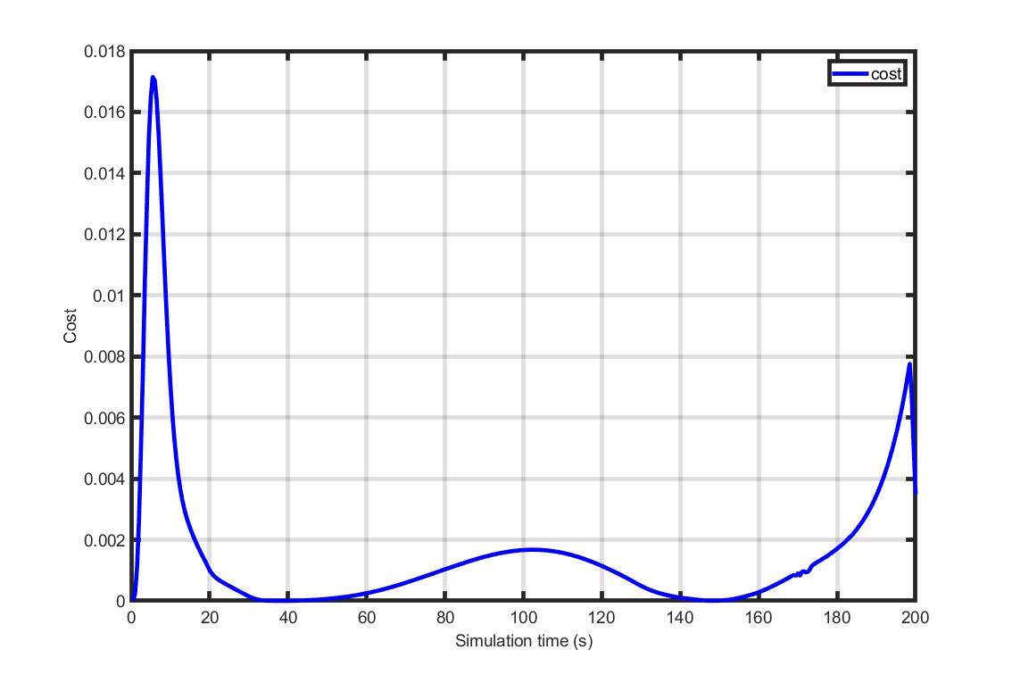
../_images/cstr_cost.png — Figure 7.1 Cost as a function of time.¶

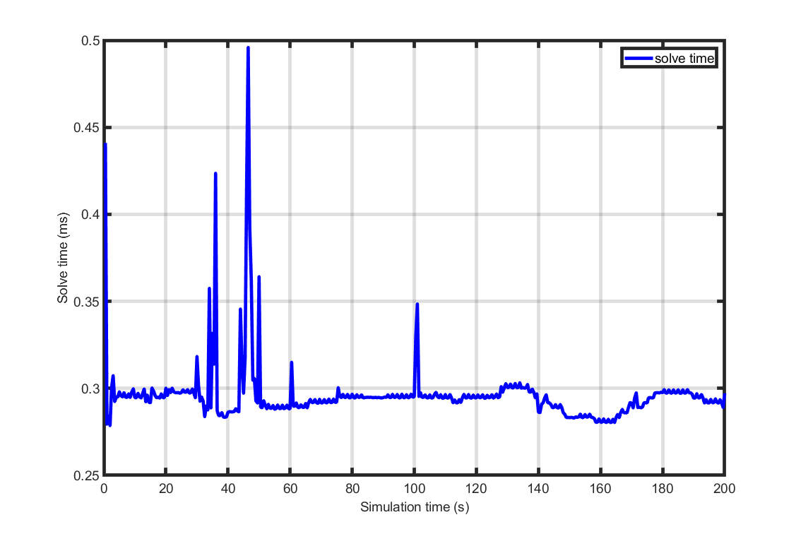
../_images/cstr_solvetime.png — Figure 7.2 Solve time as a function of simulation time.¶

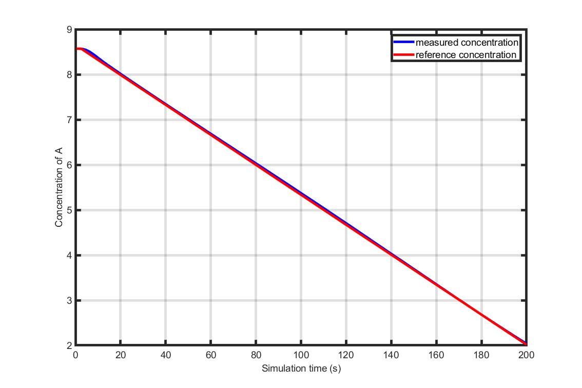
../_images/cstr_concentration.png — Figure 7.3 Concentration of $A$ as a function of simulation time.¶

7.7.2. Lane following example ¶

In this example, the use of the nlmpc plugin in Simulink is described. The example consists in making a vehicle follow a central line while keeping a user-specified velocity.

You can download the MATLAB code used in this example to try it out for yourself by clicking here.

7.7.2.1. Create an NLMPC object¶

An nlmpc object with measured and unmeasured disturbance is first created.

nlobj = nlmpc(7,3,'MV',[1 2],'MD',3,'UD',4);

The NMPC controller sample time, prediction horizon and control horizon are then specified.

nlobj.Ts = Ts;
nlobj.PredictionHorizon = 10;
nlobj.ControlHorizon = 2;

The dynamics are provided as a function name.

nlobj.Model.StateFcn = 'LaneFollowingStateFcn';

The output variables returned by LaneFollowingOutputFcn are the longitudinal velocity, the lateral deviation and the sum of the yaw angle and yaw angle output disturbance

nlobj.Model.OutputFcn = 'LaneFollowingOutputFcn';

Bound constraints are set on the manipulated (input) variables.

nlobj.MV(1).Min = -3;      % Maximum acceleration 3 m/s^2
nlobj.MV(1).Max = 3;       % Minimum acceleration -3 m/s^2
nlobj.MV(2).Min = -1.13;   % Minimum steering angle -65
nlobj.MV(2).Max = 1.13;    % Maximum steering angle 65

Scaling factors are incorporated on output and manipulated variables to optimize solver performance.

nlobj.OV(1).ScaleFactor = 15;   % Typical value of longitudinal velocity
nlobj.OV(2).ScaleFactor = 0.5;  % Range for lateral deviation
nlobj.OV(3).ScaleFactor = 0.5;  % Range for relative yaw angle
nlobj.MV(1).ScaleFactor = 6;    % Range of steering angle
nlobj.MV(2).ScaleFactor = 2.26; % Range of acceleration
nlobj.MD(1).ScaleFactor = 0.2;  % Range of Curvature

Weights on outputs and the rates of manipulated variables are set in the NLMPC object objective function.

nlobj.Weights.OutputVariables = [1 1 0];

%%
% Penalize acceleration change more for smooth driving experience.
nlobj.Weights.ManipulatedVariablesRate = [0.3 0.1];

A nonlinear interior-point FORCESPRO solver is generated from a customizable options structure.

options = nlmpcToForcesOptions();
% Set solver name
options.SolverName = 'LaneFollowSolver';
% Choose solver type 'InteriorPoint' or 'SQP'
options.SolverType = 'InteriorPoint';
% x0 and u0 are used to create a primal initial guess
options.x0 = x0;
options.mv0 = u0;
tm = tic;
[coredata, onlinedata] = nlmpcToForces(nlobj,options);
tBuild = toc(tm);

The FORCESPRO NLMPC Simulink block can then be used seamlessly. It is available in the Simulink Library Browser in the Model Predictive Control Toolbox section, as shown in Figure Figure 7.4.

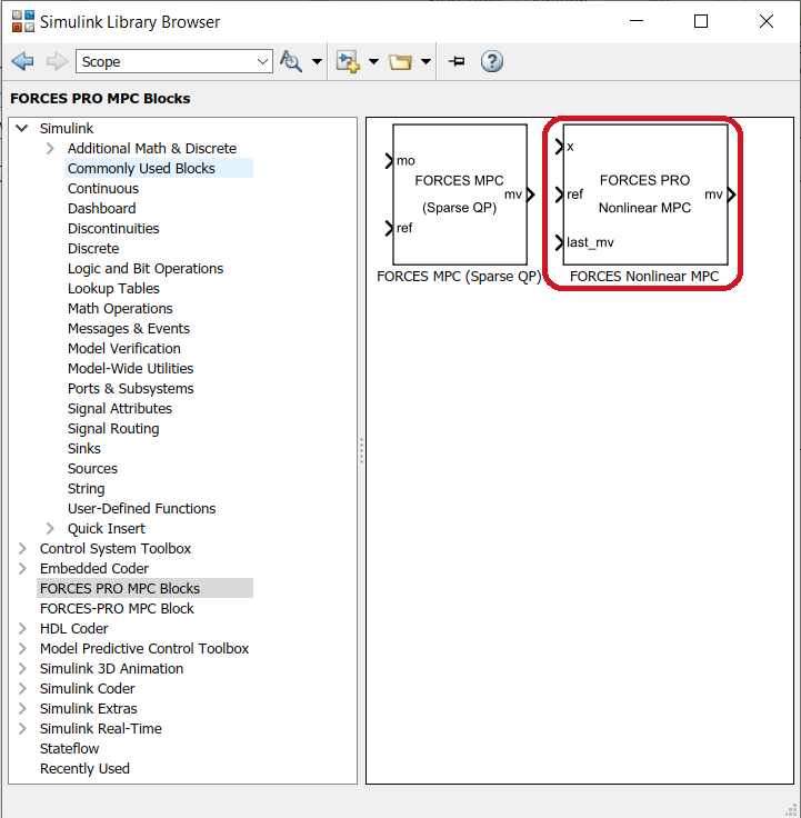
../_images/nlmpcBlockSimBrowser.PNG — Figure 7.4 FORCESPRO NMPC block.¶

In order to run the nonlinear interior-point solver, the coredata structure returned by nlmpcToForces must be provided in the block mask, as shown in Figure Figure 7.5.

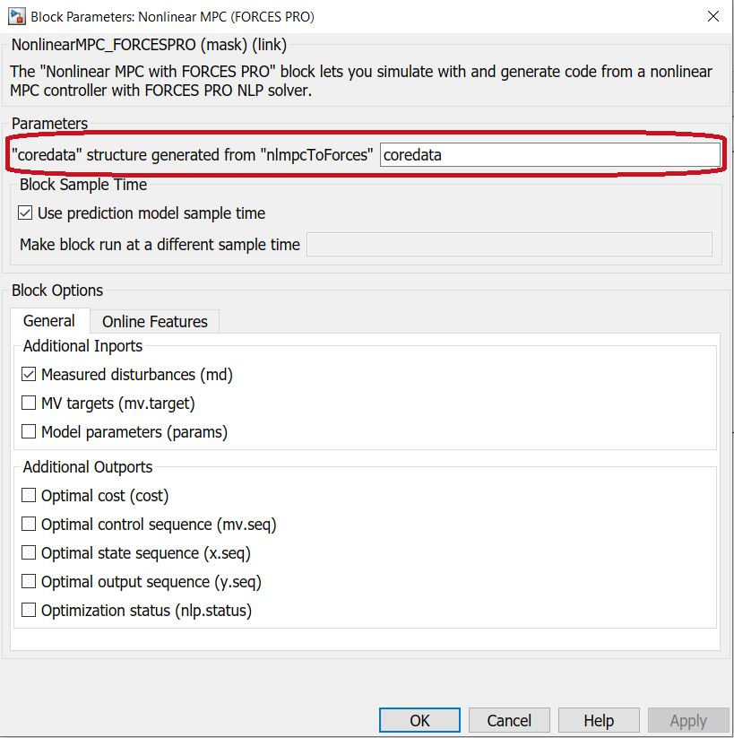
../_images/nmpcSimBlockMask.PNG — Figure 7.5 FORCESPRO NMPC block mask.¶

The Simulink model can finally be run using the sim command.

sim('LaneFollowingNMPC')

Results are shown in Figures Figure 7.6 and Figure 7.7.

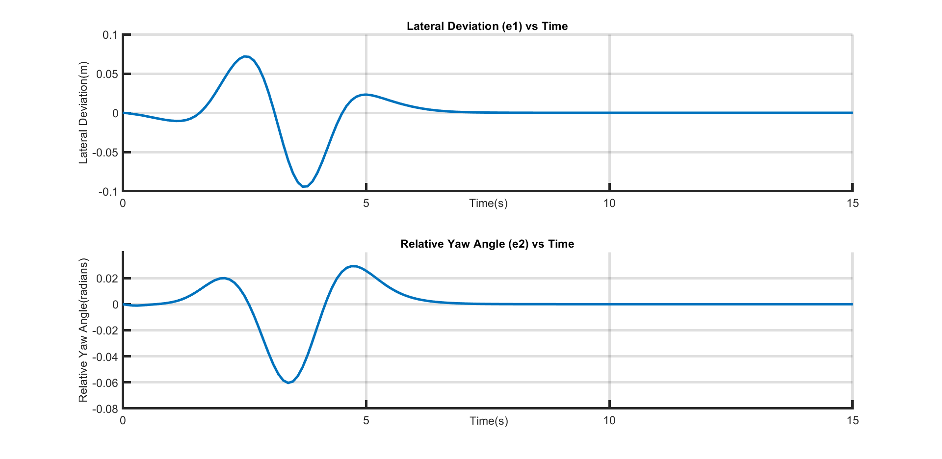
../_images/lateralDev.PNG — Figure 7.6 Vehicle lateral deviation.¶

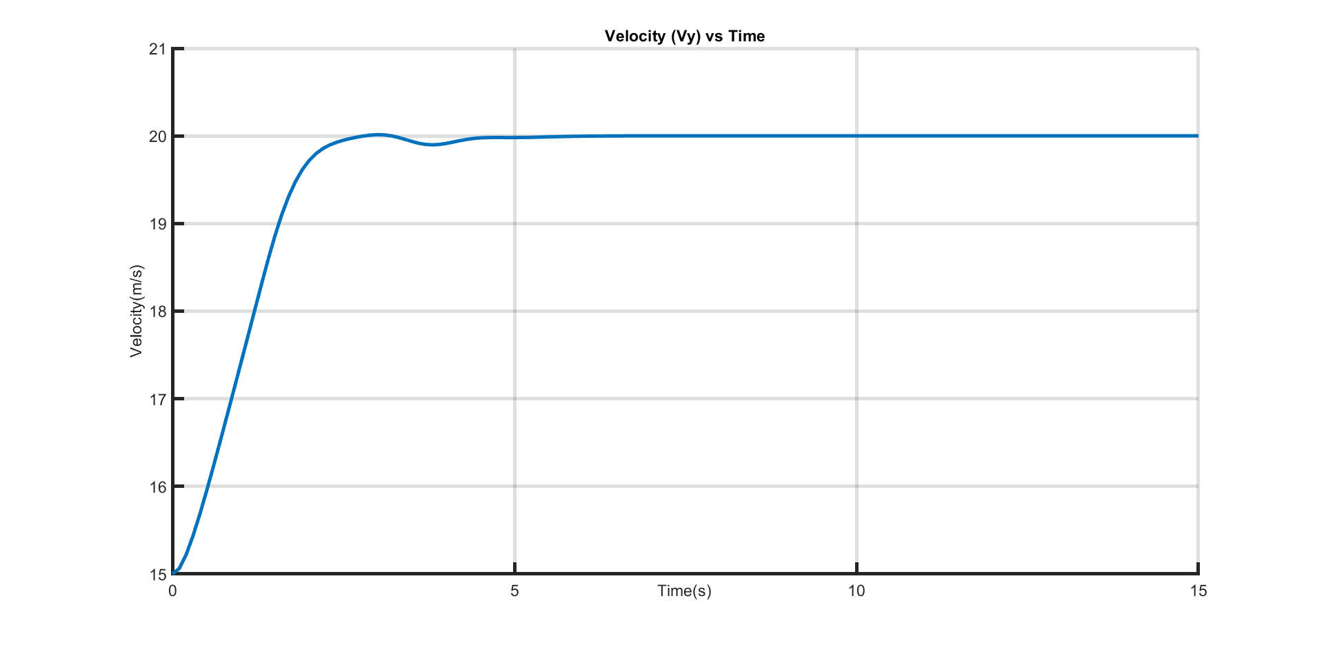
../_images/velocity.PNG — Figure 7.7 Vehicle velocity.¶

Simulink Coder (R) enables users to generate an executable from the FORCESPRO NLMPC block, so that it can be deployed for real-time applications.

7.7.2.2. Deploying the Lane Following Model on Speedgoat¶

The lane following model in Figure Figure 7.8 can be easily deployed on Speedgoat platforms by means of the code below.

% Choose Speedgoat x86 platform to run FORCESPRO solver
options.ForcesTargetPlatform = 'Speedgoat-x86';
% x0 and u0 are used to create a primal initial guess
options.x0 = x0;
options.mv0 = u0;
% Generate FORCESPRO solver
tm = tic;
[coredata, onlinedata] = nlmpcToForces(nlobj,options);
tBuild = toc(tm);

%%
% Start code generation for Speedgoat x86
mdl = 'LaneFollowingNMPC_Speedgoat_x86';
open_system(mdl);                               % Open Simulink(R) Model
load_system(mdl);                               % Load Simulink(R) Model
rtwbuild(mdl);                                  % Start Code Generation

% Deploy application from the start
tg = slrt;
if(~strcmpi(tg.Application, 'loader'))
    tg.unload();
end
tg.load(mdl);

% Execute application
tg.start();
while(strcmpi(tg.Status, 'running'))
    pause(Ts);
end
scope1 = tg.getscope(1);
scope2 = tg.getscope(2);
scope3 = tg.getscope(3);

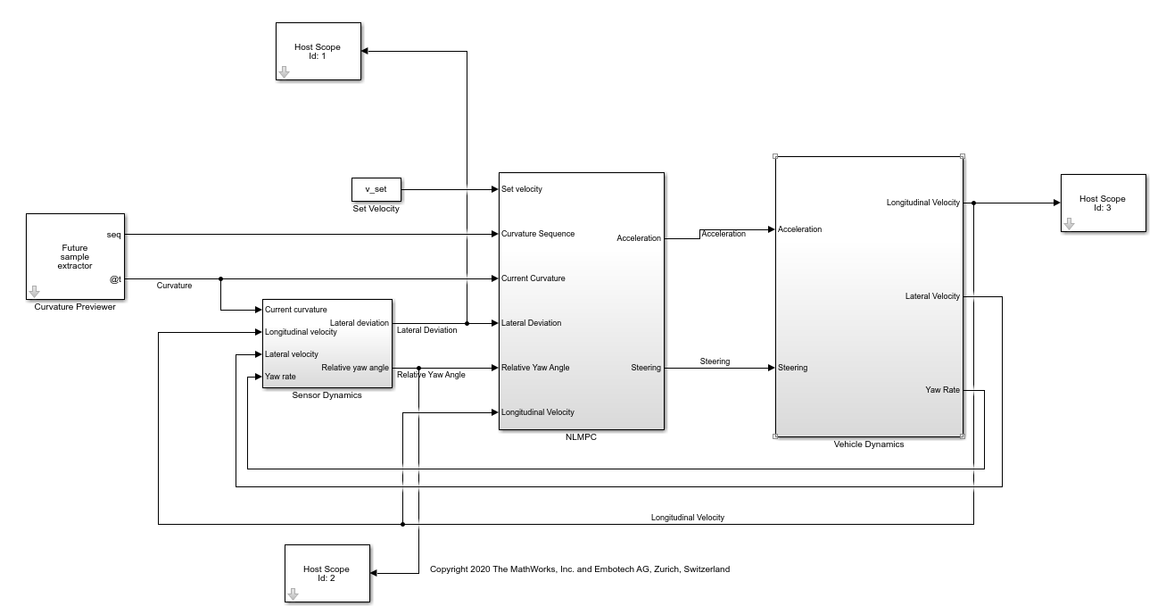
../_images/laneFollowSpeedgoatModel.PNG — Figure 7.8 Simulink Real-Time Lane Following model for Speedgoat deployment.¶

All the files necessary to run this example can be downloaded here.

7.7.3. Rocket landing example ¶

In this example we consider the motion planning problem of landing a rocket safely. The FORCESPRO solver is generated using a NLMPCMultistage object. We will cover the details of the model below. For further details, see here.

You can download the MATLAB code used in this example to try it out for yourself by clicking here.

7.7.3.1. The dynamical model¶

The model we consider is a first-principles nonlinear dynamical model. The state $x$ of our system is $6$-dimensional while the control $u$ is $2$-dimensional. The interpretation of the different states/control inputs is given as follows:

\begin{align*} u_1&: \ \text{Left thrust} \quad (N) \\ u_2&: \ \text{Right thrust} \quad (N) \\ x_1&: \ \text{Horizontal position of the center of gravity} \quad (m) \\ x_2&: \ \text{Vertical position of the center of gravity} \quad (m) \\ x_3&: \ \text{Tilt with respect to the center of gravity} \quad (r) \\ x_4&= \tfrac{dx_1}{dt} \quad (\tfrac{m}{s}) \\ x_5&= \tfrac{dx_2}{dt} \quad (\tfrac{m}{s}) \\ x_6&= \ \text{Angular velocity} \quad (\tfrac{r}{s}) \end{align*}

The differential equation governing the dynamics is given by

\begin{align*} \dot{x}_1 &= x_4 \\ \dot{x}_2 &= x_5 \\ \dot{x}_3 &= x_6 \\ \dot{x}_4 &= \frac{-\sin(x_3)(u_1 + u_2)}{m} \\ \dot{x}_5 &= \frac{\cos(x_3)(u_2 - u_1)}{m} - g \\ \dot{x}_6 &= \frac{2 L_2 ( u_2 - u_1 )}{m L_1^2}, \end{align*}

where we use of the following constants:

Name

Value

Description

$L_1$

$10m$

Center of gravity to top/bottom end

$L_2$

$5m$

Center of gravity to left/right end

$m$

$1kg$

Mass of rocket

$g$

$9.806 \tfrac{m}{s^2}$

Gravitational constant

Name	Value	Description
\(L_1\)	\(10m\)	Center of gravity to top/bottom end
\(L_2\)	\(5m\)	Center of gravity to left/right end
\(m\)	\(1kg\)	Mass of rocket
\(g\)	\(9.806 \tfrac{m}{s^2}\)	Gravitational constant

7.7.3.2. Constructing a NLMPCMultistage object¶

The first step to generate a FORCESPRO solver is to construct a nlmpcMultistage object and set the constraints on our manipulated variables (MV) and states (State).

% Construct nlmpcMultistage object and set dynamics
Ts = 0.2;
pPlanner = 50;
planner = nlmpcMultistage(pPlanner,6,2);
planner.Ts = Ts;

% Limit thrusts between 0 and 8 Newton
planner.MV(1).Min = 0;
planner.MV(1).Max = 8;
planner.MV(2).Min = 0;
planner.MV(2).Max = 8;

% Specify lower bound on y-axis to avoid crashing
planner.States(2).Min = 10;

Then we specify the state transition function along with a cost function for every stage. Note that these functions are specified via the of the function.

planner.Model.StateFcn = 'RocketStateFcn';
for ct=1:pPlanner
    planner.Stages(ct).CostFcn = 'RocketPlannerCostFcn';
end

7.7.3.3. Specifying solver options and generating a solver¶

Once we have defined our nlmpcMultistage object planner we need to specify information about the solver we would like to generate. This can be done through the options generated by nlmpcMultistageToForcesOptions

%% Generate FORCES NLP Solver
options = nlmpcMultistageToForcesOptions;
options.Server = 'https://forces.embotech.com/';
options.x0 = x0;
options.mv0 = u0;
options.UseOnlineConstraintMVMin = true;
options.UseOnlineConstraintMVMax = true;
options.UseOnlineConstraintStateMin = true;

With both our options and nlmpcMultistage object at hand we can go ahead and generate the FORCESPRO solver:

[coredata, onlinedata, model] = nlmpcMultistageToForces(planner, options);

7.7.3.4. Results¶

In plot Figure 7.9 the optimal trajectory for landing the rocket is displayed. As can be observed in the generated animation which appears when running the code (see Figure 7.10), the FORCESPRO solver manages to control the rocket and land it safely.

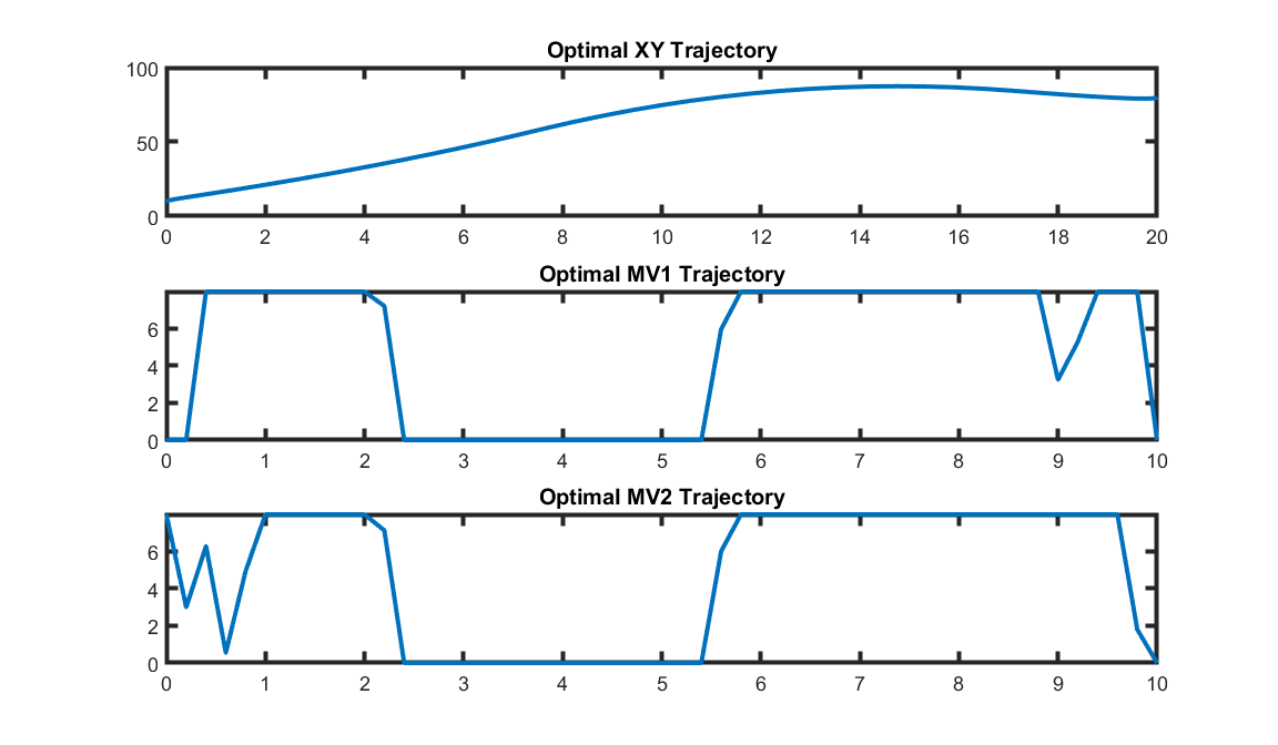
../_images/rocket_lander_plot.png — Figure 7.9 Optimal rocket trajectory.¶

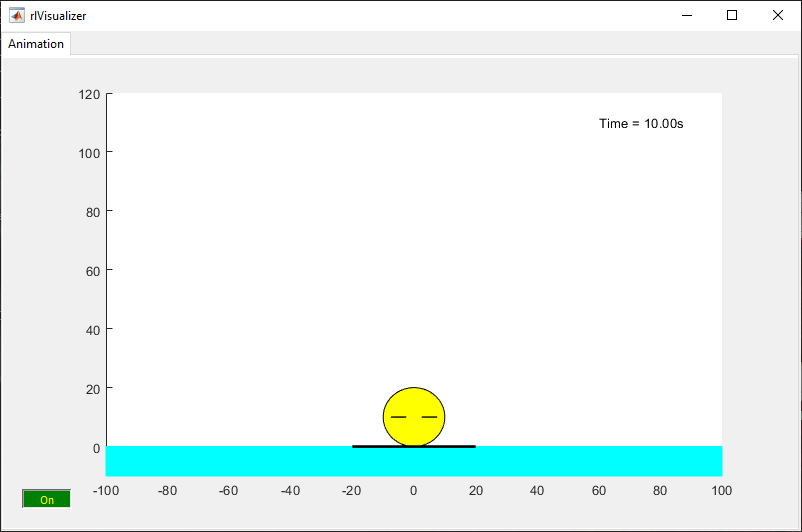
../_images/rocket_lander_animation.PNG — Figure 7.10 Rocket lander animation generated when running the rocket lander example.¶

Input	Description
coredata	A structure containing the constant controller settings. It is generated by the `nlmpcToForces` method and used as a constant
x	A \(n_x\)-by-1 column vector, representing the current prediction model states
lastMV	A \(nmv\)-by-1 column vector, representing the control action applied to the plant at the previous control interval
onlinedata	A structure containing run time signals