13.3. dSPACE deployment through ConfigurationDesk

This process applies to the following dSPACE platforms

• dSPACE MicroAutoBox III

• dSPACE SCALEXIO

Important

When deploying to a target hardware platform, the library included in the lib_target directory of the generated solver should be used instead of the library in the lib directory.

13.3.1. Code Generation

The steps to deploy a FORCESPRO controller on a dSPACE platform are detailed below.

1. (Figure 13.28) Set the code generation options:

When generating code for HW target platforms, codeoptions.platform needs to be set.

• dSPACE MicroAutoBox III: 'dSPACE-MABXIII'

• dSPACE SCALEXIO: 'dSPACE-SCALEXIO'

codeoptions.platform = '<platform_name>'; % to generate code for the dSPACE platform
codeoptions.printlevel = 0; % printing should be disabled on target HW
codeoptions.cleanup = 0; % to keep necessary files for target compile

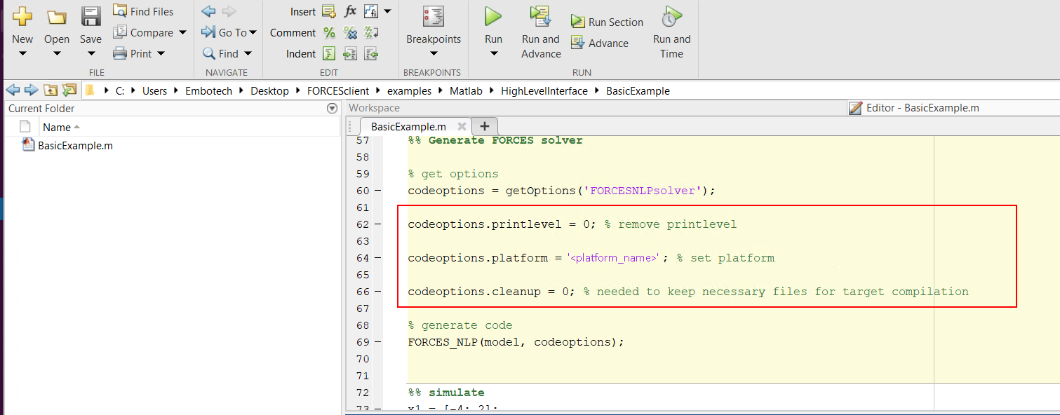
Figure 13.28 Set the appropriate code generation options.

1. Create a new Simulink model (henceforth referred to as dSPACE.slx) using the dSPACE Run-Time Target template provided by dSPACE and save it in the BasicExample folder (see Figure 13.29).

2. Populate the Simulink model with the system you want to control (see Figure 13.30).

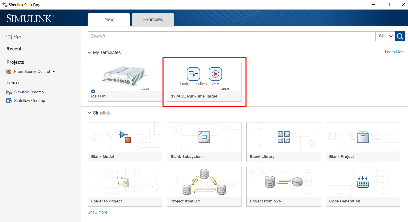
Figure 13.29 Create a Simulink model.

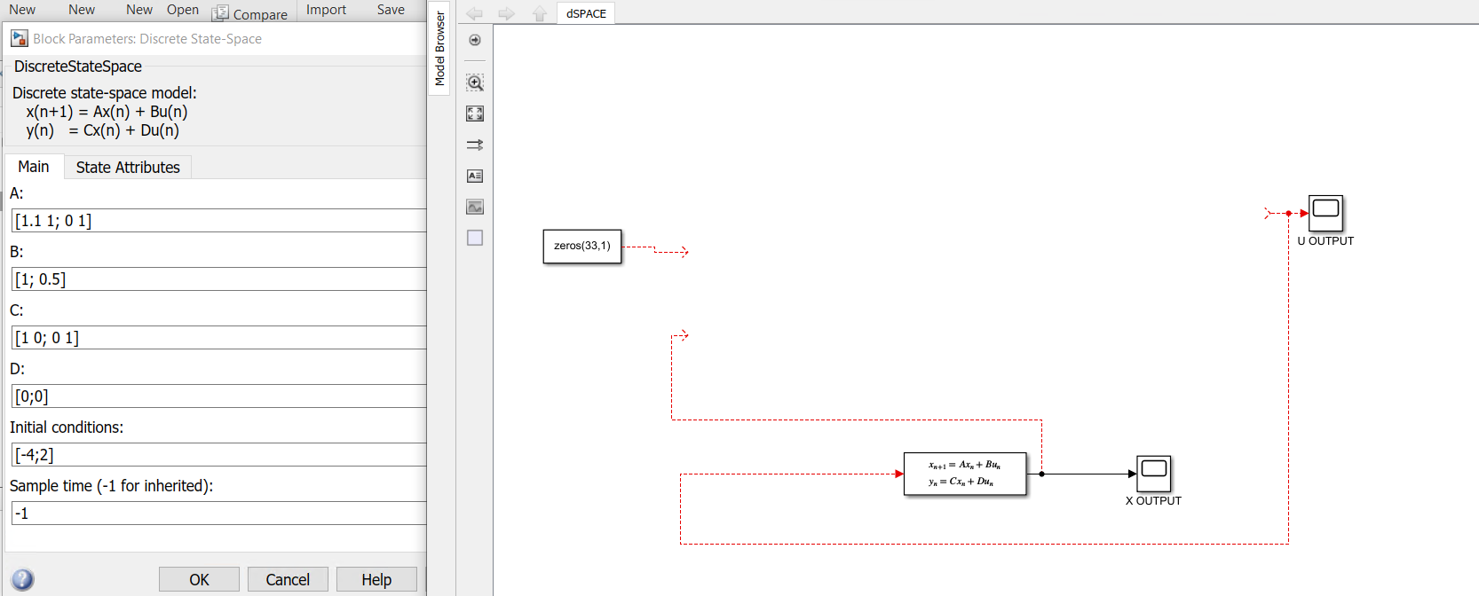
Figure 13.30 Populate the Simulink model.

4. Run the BasicExample.m script to perform code generation for your solver (henceforth referred to as FORCESNLPsolver, placed in the folder “BasicExample”). This will create the necessary files for your building (see Figure 13.31 , Figure 13.32 and Figure 13.33).

5. The FORCESNLPsolver_simulinkBlock.<mex_extension> file (created during code generation) needs to be in the same path as your model (see Figure 13.34).

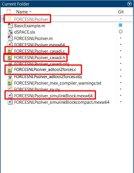
Figure 13.31 Generated files.

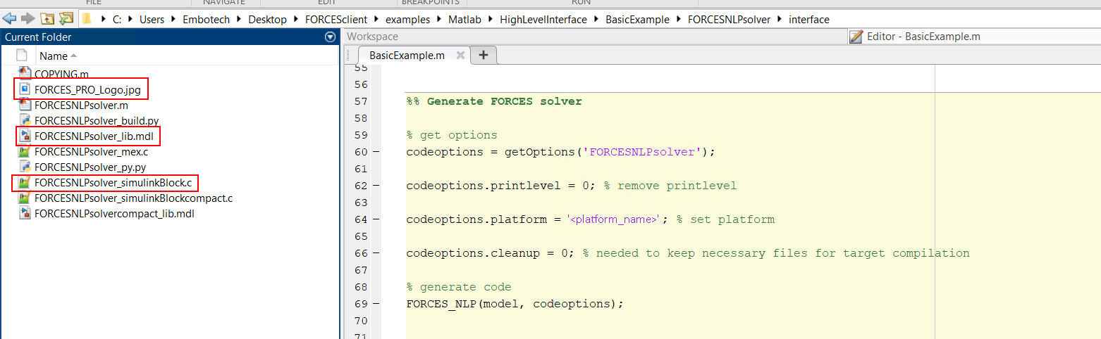
Figure 13.32 Solver interface files.

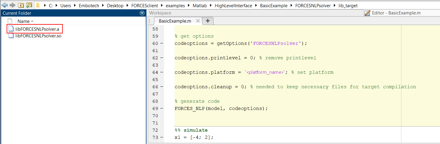
Figure 13.33 Solver libraries.

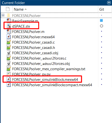
Figure 13.34 The .<mex_extension> solver file is in the same path as the model.

6. Open the FORCESNLPsolver_lib.mdl Simulink model file, contained in the interface folder of the FORCESNLPsolver folder created during code generation (see Figure 13.35).

7. Copy-paste the FORCESPRO Simulink block into your simulation model and connect its inputs and outputs appropriately (see Figure 13.36).

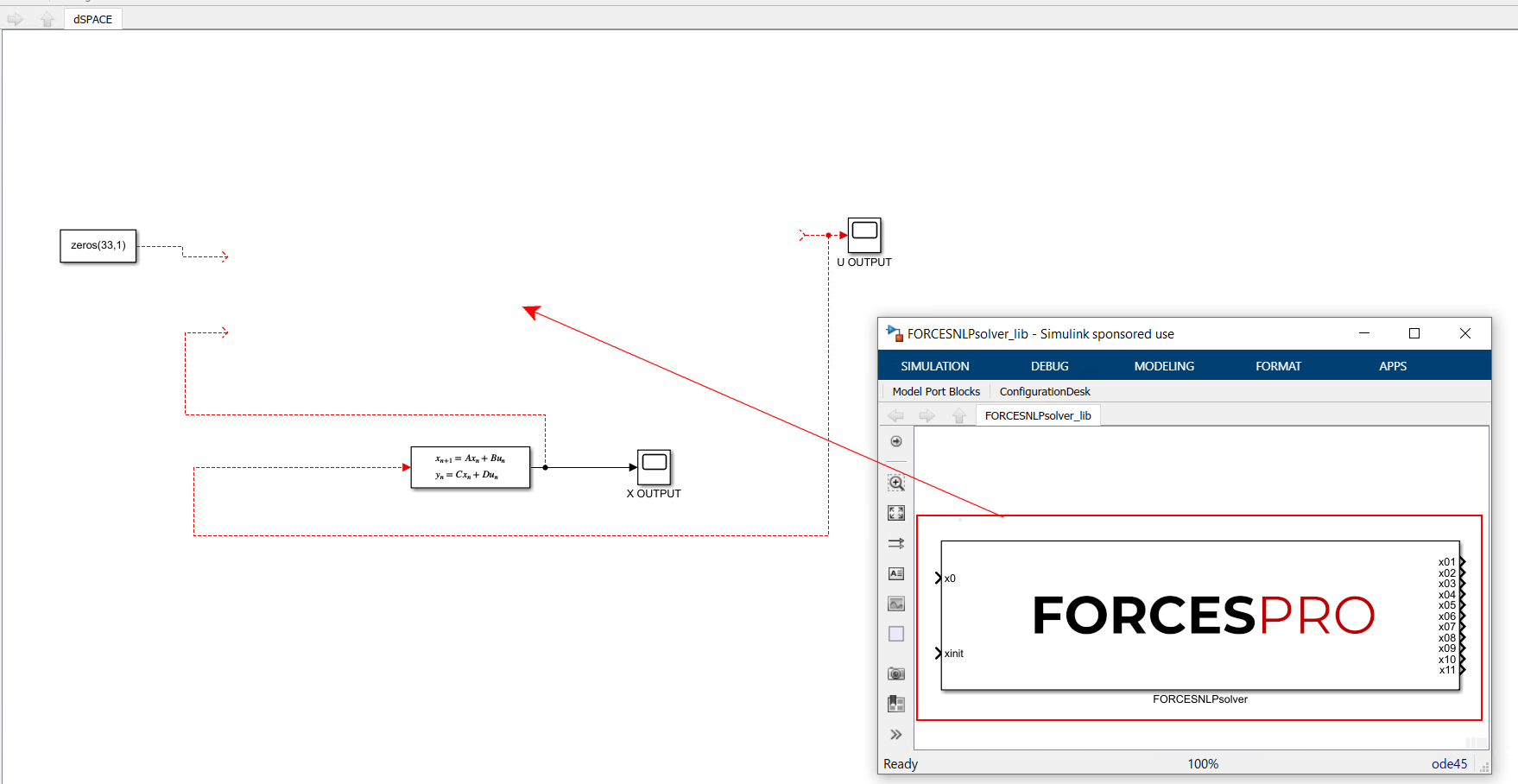
Figure 13.35 Open the generated Simulink solver model.

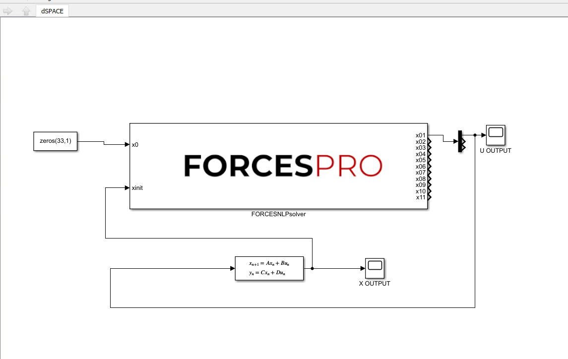
Figure 13.36 Copy-paste and connect the FORCESPRO block.

8. Access the Simulink model’s options. In the “Solver” tab, set the options (see Figure 13.37):

• Simulation start/stop time: Depending on the simulation wanted.

• Solver type: Discrete or fixed-step.

• Fixed-step size: Needs to be higher than the execution time of the solver.

9. In the “Code Generation” tab, set the options (see Figure 13.38):

• System target file: dsrt.tlc

• Language: C / C++

• Generate makefile: Checked

• Template makefile: dsrt_default_tmf

• Make command: make_dsrt

10. In the “Code Generation/Custom Code” tab, include the directories (see Figure 13.39):

• .\FORCESNLPsolver\include

• .\FORCESNLPsolver\interface

• .\FORCESNLPsolver\lib_target

11. In the “Code Generation/Custom Code” tab, add the source files (see Figure 13.40):

• FORCESNLPsolver_simulinkBlock.c

• FORCESNLPsolver_adtool2forces.c

• FORCESNLPsolver_casadi.c

12. In the “Code Generation/Custom Code” tab, add the library file (see Figure 13.41):

• libFORCESNLPsolver.a

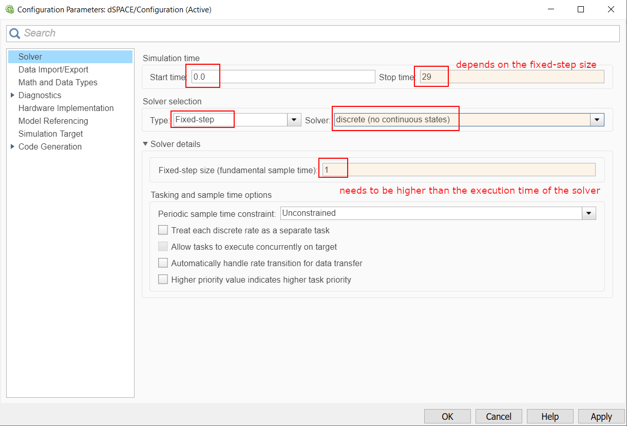
Figure 13.37 Set the Simulink solver options.

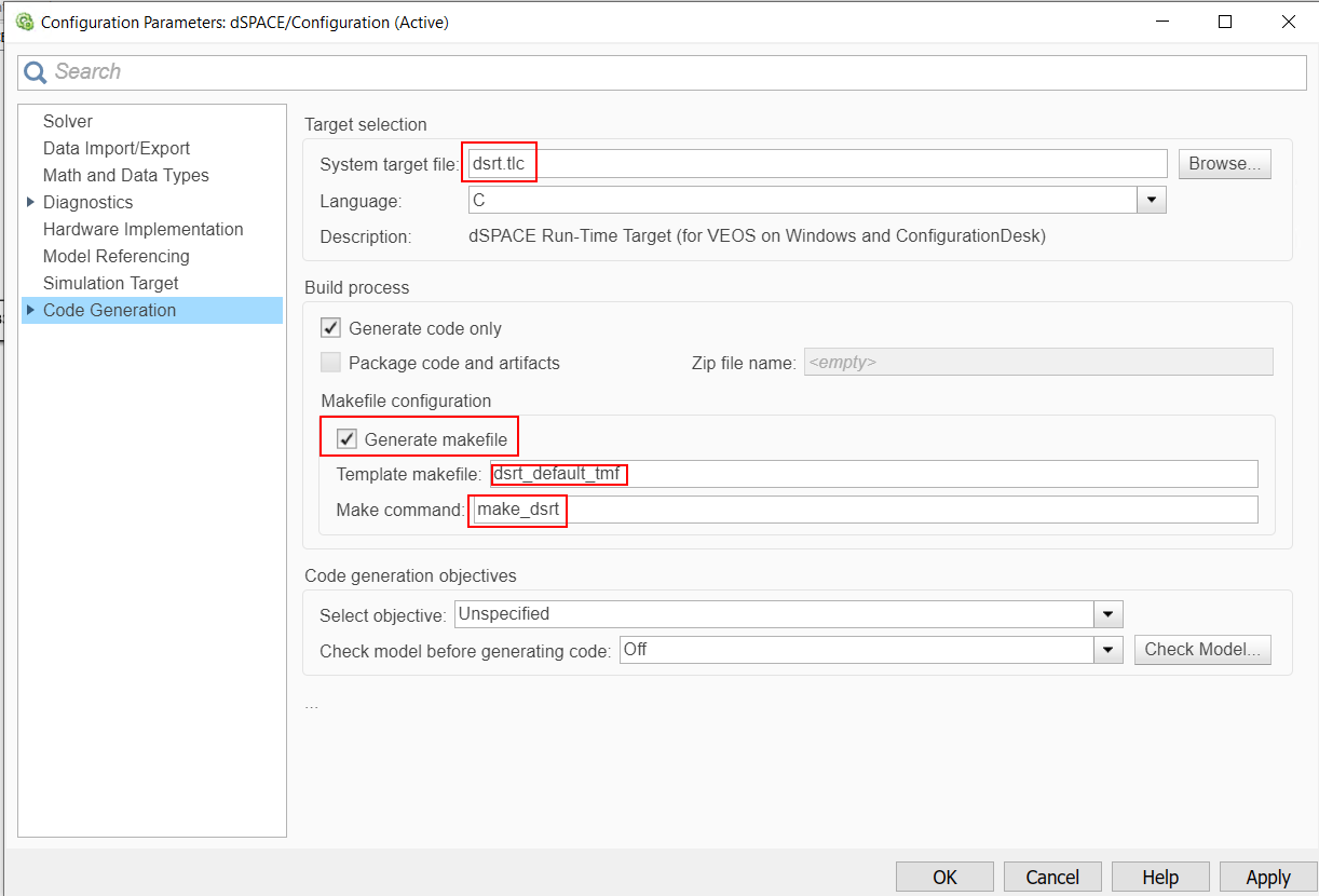
Figure 13.38 Set the Simulink code generation options.

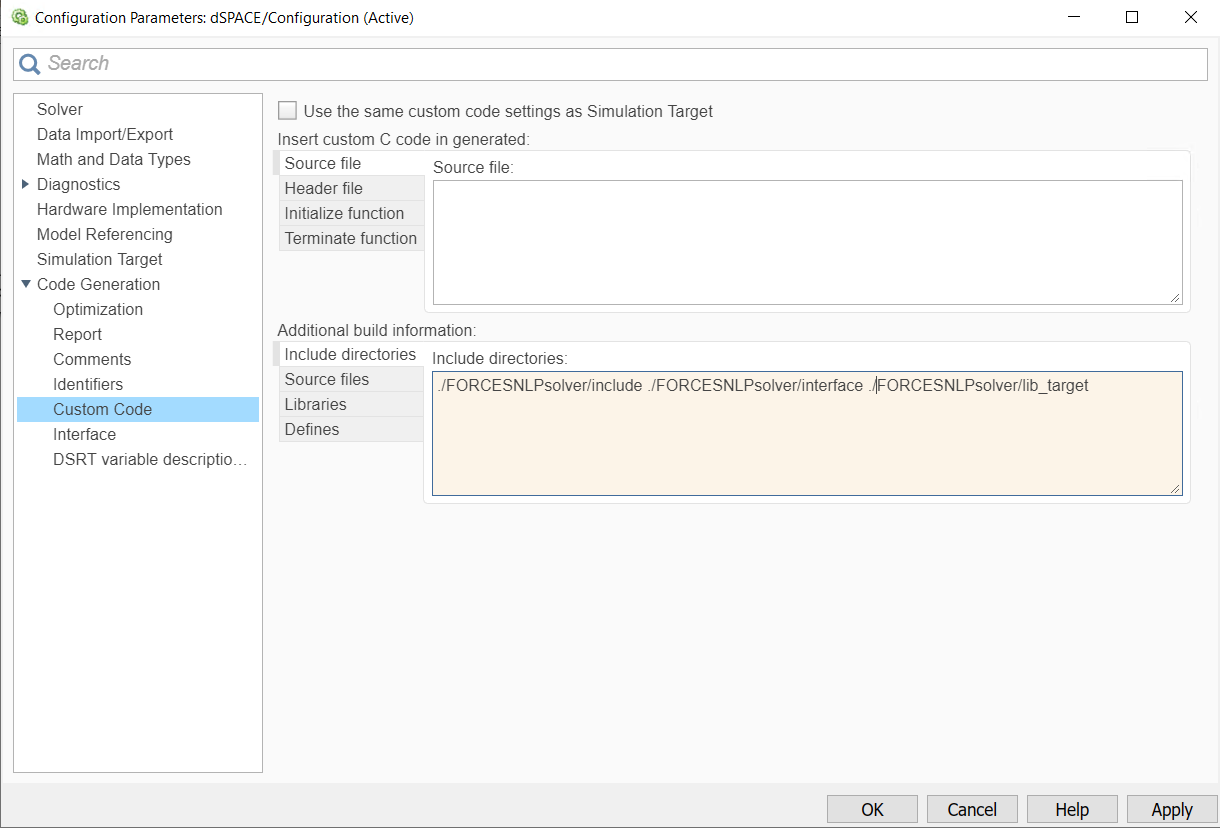
Figure 13.39 Add the directories included for the code generation.

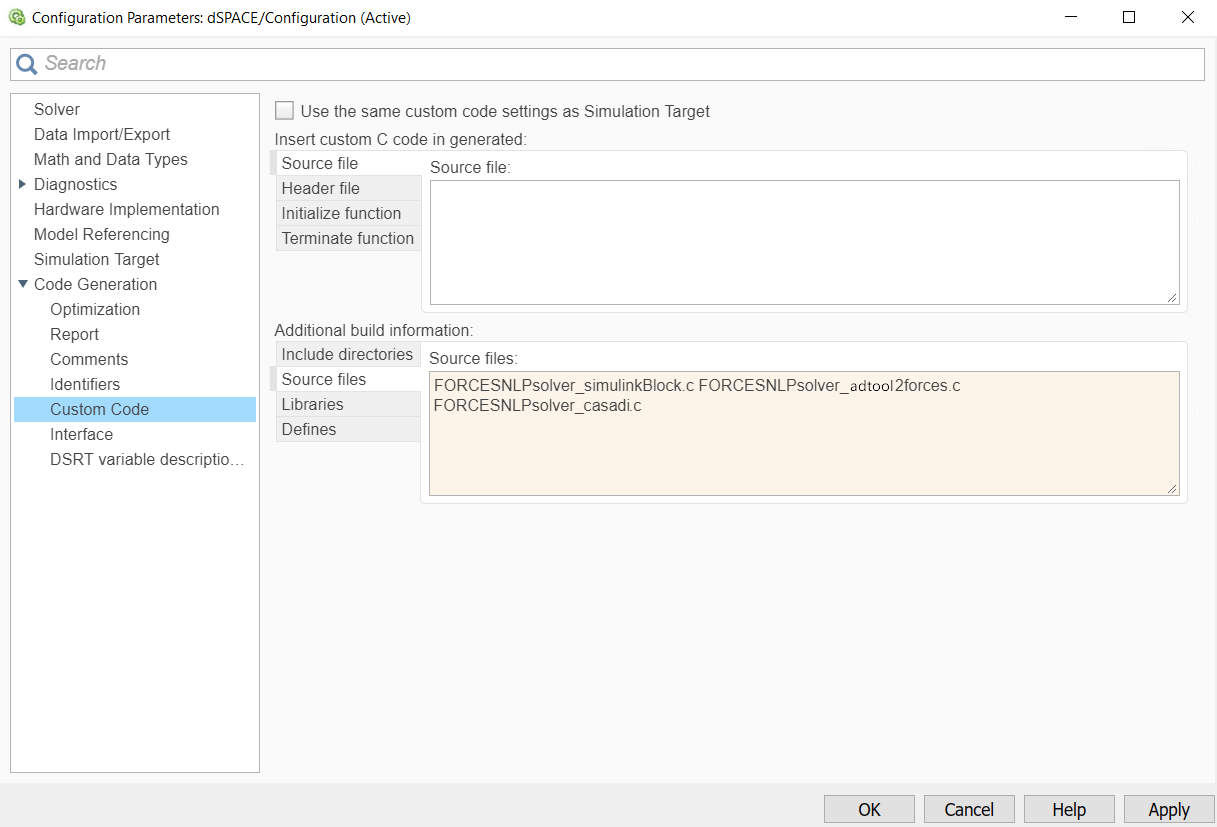
Figure 13.40 Add the source files used for the code generation.

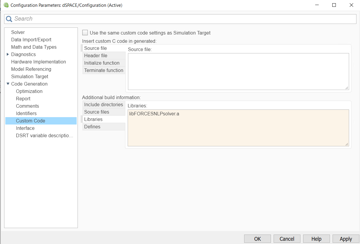
Figure 13.41 Add the libraries used for the code generation.

13. Access the FORCESPRO block’s parameters (see Figure 13.42).

14. Remove the “FORCESNLPsolver” prefix from the S-function module (see Figure 13.43).

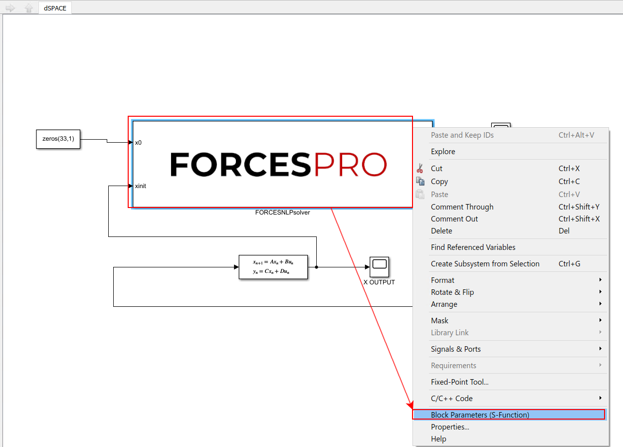
Figure 13.42 Open the FORCESPRO block’s parameters.

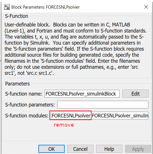
Figure 13.43 Remove the leading solver name from the S-function module.

15. Create a new Project and Application in ConfigurationDesk. Select directory of project, name of project and application, the model dSPACE.slx as the application process and connected dSPACE platform to deploy to (see Figure 13.44).

16. Go to the tasks tab and make sure the period of the Periodic Task matches the fixed step size selected in the Simulink model options (see Figure 13.45).

17. Go to the build tab and start the building process. After building is complete the application will be loaded automatically in the dSPACE platform (see Figure 13.46).

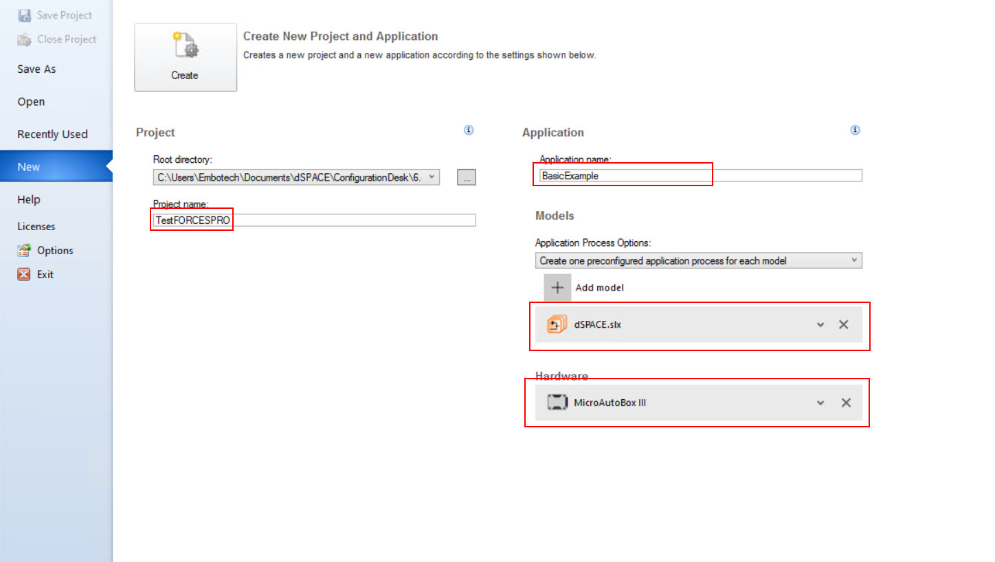
Figure 13.44 Create project and application in ConfigurationDesk.

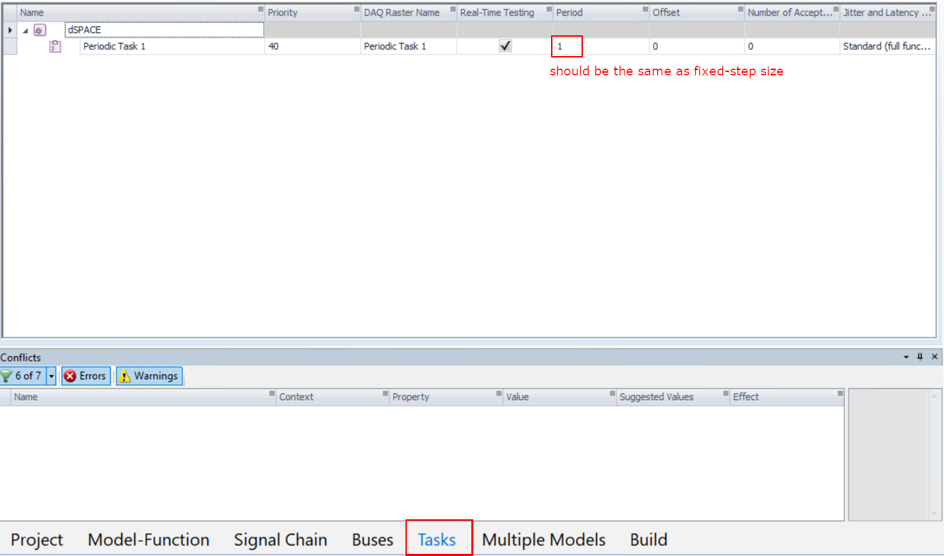
Figure 13.45 Set period of Periodic Task.

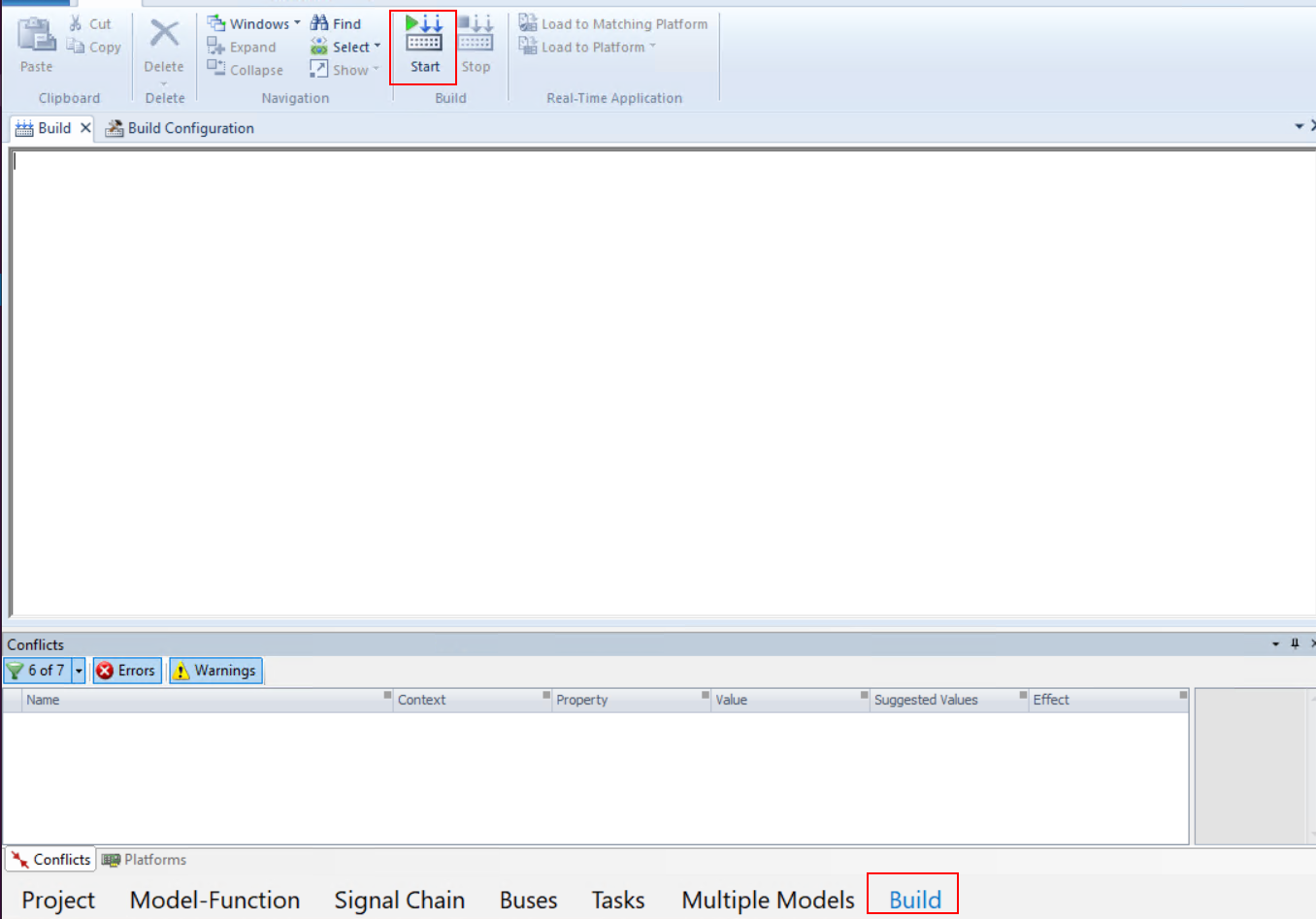
Figure 13.46 Build the project.

13.3.2. Solver Execution

The steps to simulate a FORCESPRO controller on a dSPACE platform are detailed below.

1. After code generation with FORCESPRO and building with the ConfigurationDesk, the ConfigurationDesk project will have generated files to use to run your model on the dSPACE platform (see Figure 13.47 and Figure 13.48).

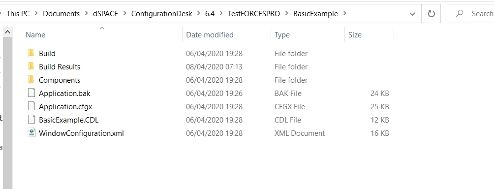
Figure 13.47 The generated files from the ConfigurationDesk building.

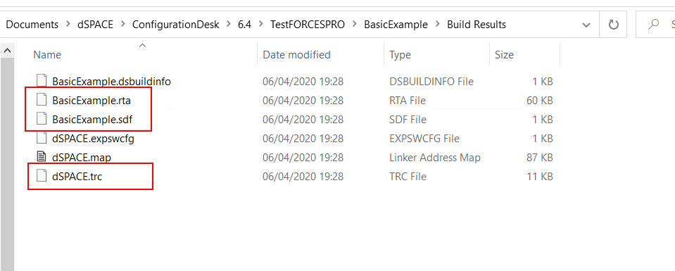
Figure 13.48 The files necessary for the simulation of the FORCESPRO controller.

2. Open dSPACE Control Desk and select create new project and name it (see Figure 13.49).

3. Name the experiment to execute (see Figure 13.50).

4. Select the platform to which you will deploy the generated executable (see Figure 13.51).

5. Import the variable description file BasicExample.sdf in order to have access to the model variables and see the results of the execution (see Figure 13.52).

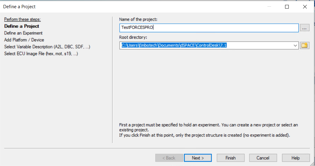
Figure 13.49 Start a new project and name it.

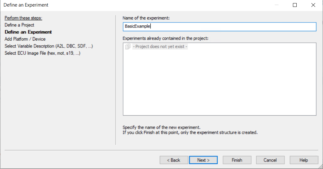
Figure 13.50 Name your experiment.

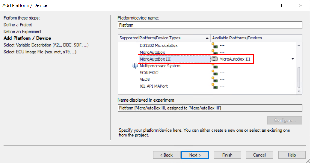
Figure 13.51 Select the dSPACE platform.

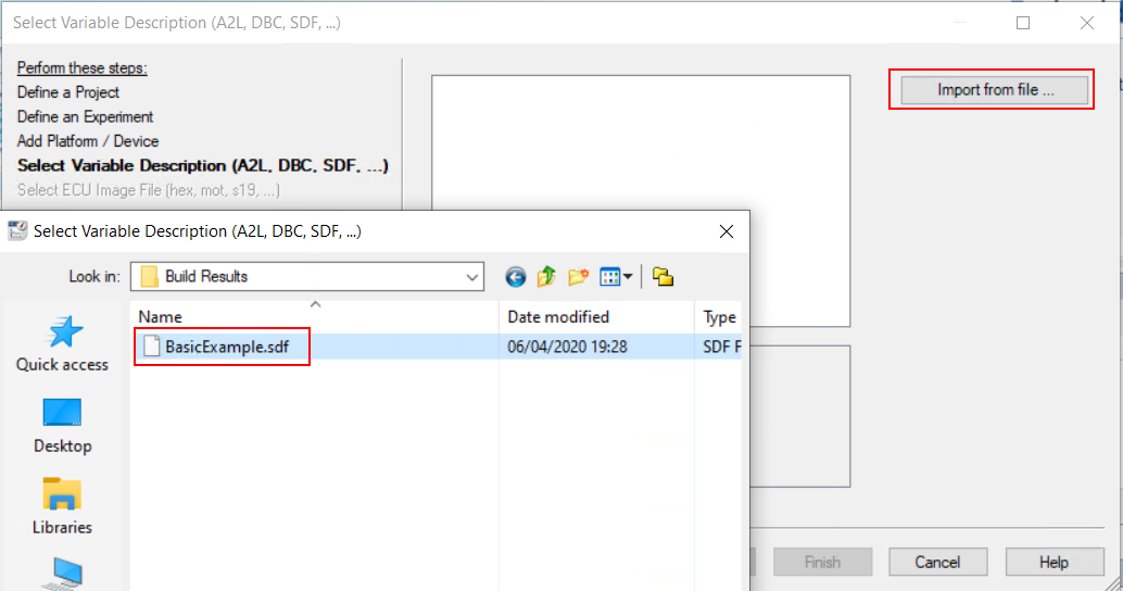
Figure 13.52 Import the variable description file.

6. On the project layout select the tab Variables and on the BasicExample.sdf category expand Model Root.

7. Select U OUTPUT and X OUTPUT and Drag & Drop all the input variables together to the Layout. In the opened menu select Time Plotter (see Figure 13.53 and Figure 13.54).

8. To see all the plots concurrently right-click on the left of the Y-axis and select YAxes-view> Horizontal stacked (see Figure 13.55).

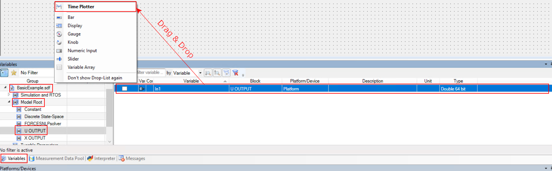
Figure 13.53 Add the inputs of U OUTPUT in a Time Plotter.

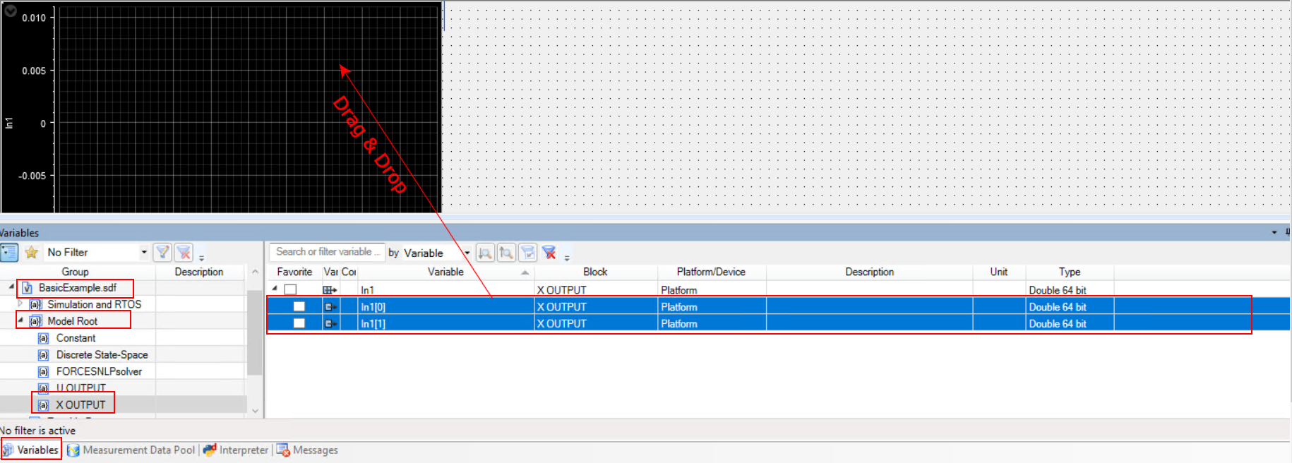
Figure 13.54 Add the inputs of X OUTPUT in the same Time Plotter.

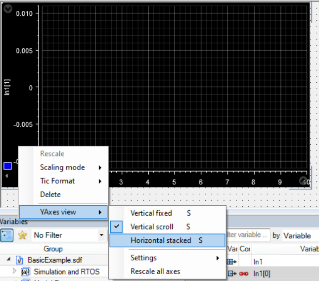
Figure 13.55 Select to show all the signals on the same plot with their own Y-axes

9. Application should have already been loaded from the building of ConfigurationDesk. Otherwise, select the Platforms/Devices tab. Right-Click on your platform and select Real-Time Application> Load. Choose the executable file BasicExample.rta (see Figure 13.56 and Figure 13.57).

10. Select Go Online and Start Measuring to see the results. (see Figure 13.58 and Figure 13.59).

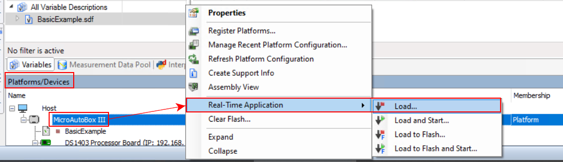
Figure 13.56 Load the application on the dSPACE platform.

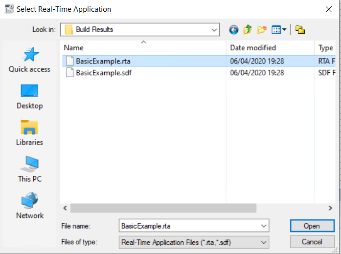
Figure 13.57 Select BasicExample.rta from the ConfigurationDesk project folder.

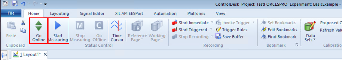
Figure 13.58 Buttons Go Online and Start Measuring to receive execution results.

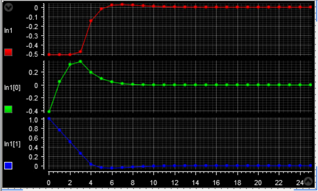
Figure 13.59 Plots and results from experiment on a dSPACE platform.