14.4. Speedgoat
Important
When deploying to a target hardware platform, the library included in the lib_target directory of the generated solver should be used instead of the library in the lib directory.
14.4.1. High-level interface
14.4.1.1. Instructions
The steps to deploy and simulate a FORCESPRO controller on a Speedgoat platform are detailed below.
(Figure 14.60) Set the code generation options:
codeoptions.platform = 'Speedgoat-x86'; % to specify the platform
codeoptions.printlevel = 0; % on some platforms printing is not supported
codeoptions.cleanup = 0; % to keep necessary files for target compile
and then generate the code for your solver (henceforth referred to as “FORCESNLPsolver”, placed in the folder “BasicExample”) using the high-level interface.
(Figure 14.61) Create a new Simulink model using the blank model template.
(Figure 14.62) Populate the Simulink model with the system you want to control.
(Figure 14.63) Make sure the
FORCESNLPsolver_simulinkBlock.mexw64file (created during code generation) is on the MATLAB path.(Figure 14.64) Open the
FORCESNLPsolver_lib.mdlSimulink model file, contained in theinterfacefolder of theFORCESNLPsolverfolder created during code generation.(Figure 14.65) Copy-paste the FORCESPRO Simulink block into your simulation model and connect its inputs and outputs appropriately.
(Figure 14.66) Access the Simulink model’s options.
(Figure 14.67) In the “Solver” tab, set the options:
Simulation start/stop time: Depending on the simulation wanted.
Solver type: Discrete or fixed-step.
Fixed-step size: Needs to be higher than the execution time of the solver.
(Figure 14.68) In the “Code Generation” tab, set the options:
System target file:
slrt.tlcLanguage: C
Generate makefile: On
Template makefile:
slrt_default_tmfMake command:
make_rtw
(Figure 14.69) In the “Code Generation/Custom Code” tab, include the directories:
BasicExample
BasicExample\FORCESNLPsolver\interface
BasicExample\FORCESNLPsolver\lib_target
(Figure 14.70) In the “Code Generation/Custom Code” tab, add the source files:
FORCESNLPsolver_simulinkBlock.c
FORCESNLPsolver_adtool2forces.c
FORCESNLPsolver_casadi.c
(Figure 14.71) In the “Code Generation/Custom Code” tab, add the library file:
FORCESNLPsolver.lib
(Figure 14.72) Access the FORCESPRO block’s parameters.
(Figure 14.73) Remove “FORCESNLPsolver” and “FORCESNLPsolver_simulinkBlock” from the S-function module.
(Figure 14.74) Compile the code of the Simulink model. This will also automatically load the model to the connected Speedgoat platform.
Deployment is complete and simulations can now be run on the Speedgoat platform.
Run the simulation on the Speedgoat platform.
You can download the MATLAB code of this simulation to try it out for yourself by clicking
here.
14.4.1.2. Figures
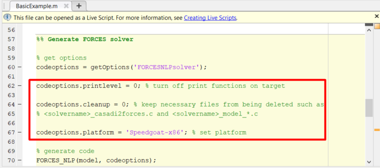
Figure 14.60 Set the appropriate code generation options.
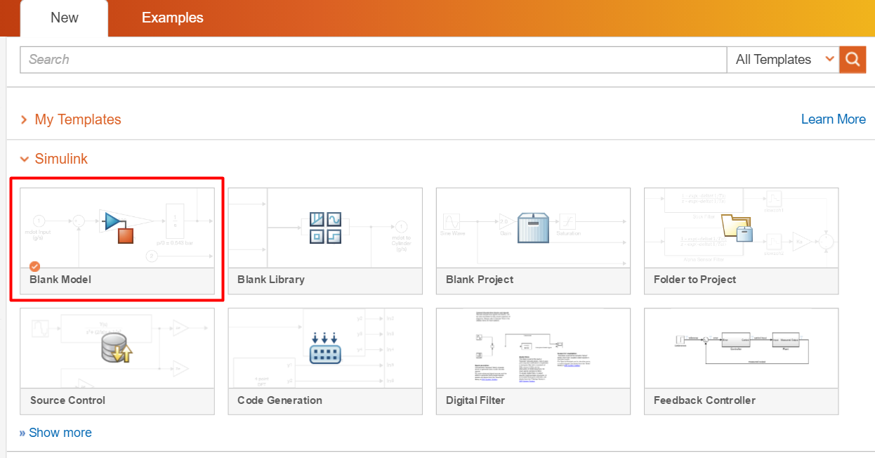
Figure 14.61 Create a Simulink model.
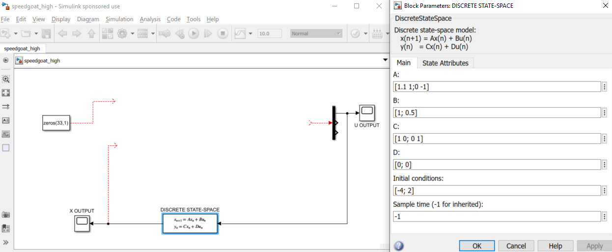
Figure 14.62 Populate the Simulink model.
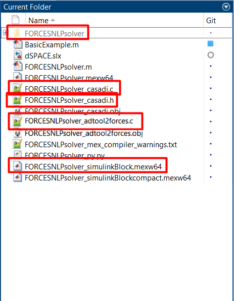
Figure 14.63 Add the folder containing the .mexw64 solver file to the MATLAB path.
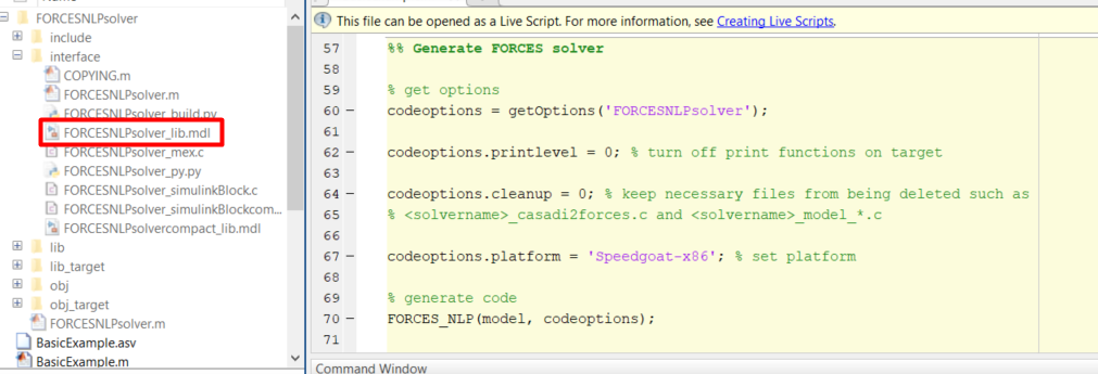
Figure 14.64 Open the generated Simulink solver model.
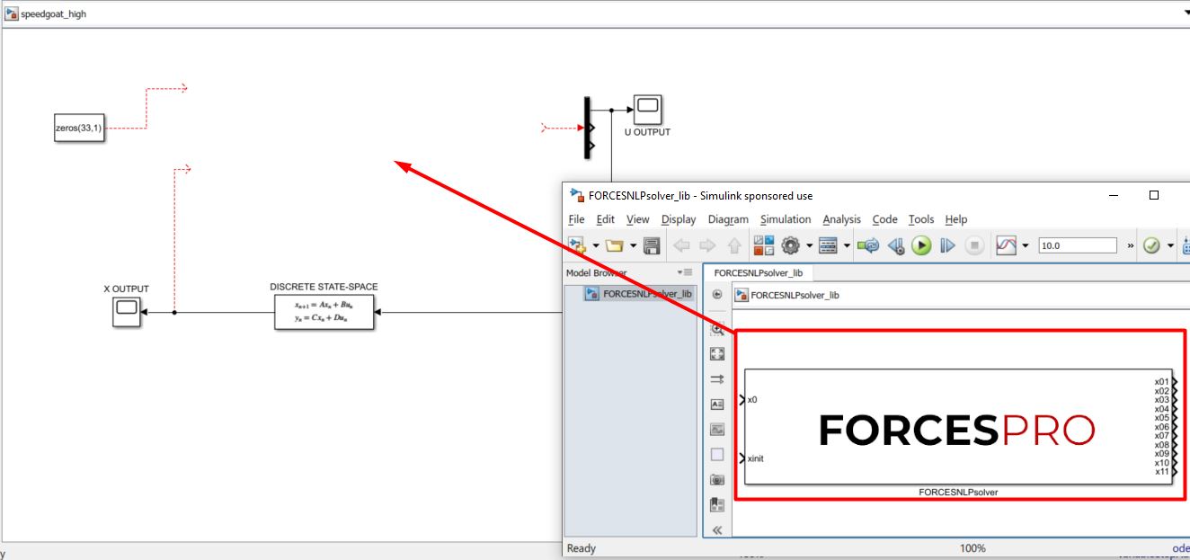
Figure 14.65 Copy-paste and connect the FORCESPRO block.
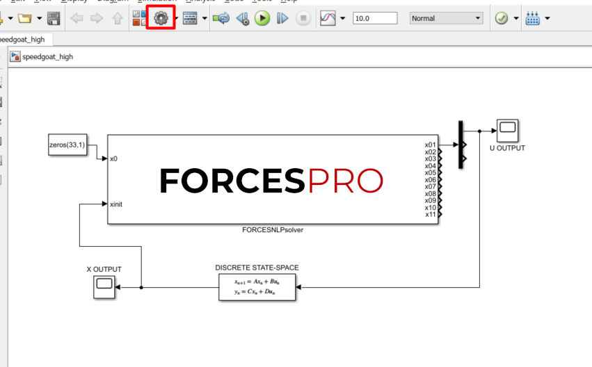
Figure 14.66 Open the Simulink model options.
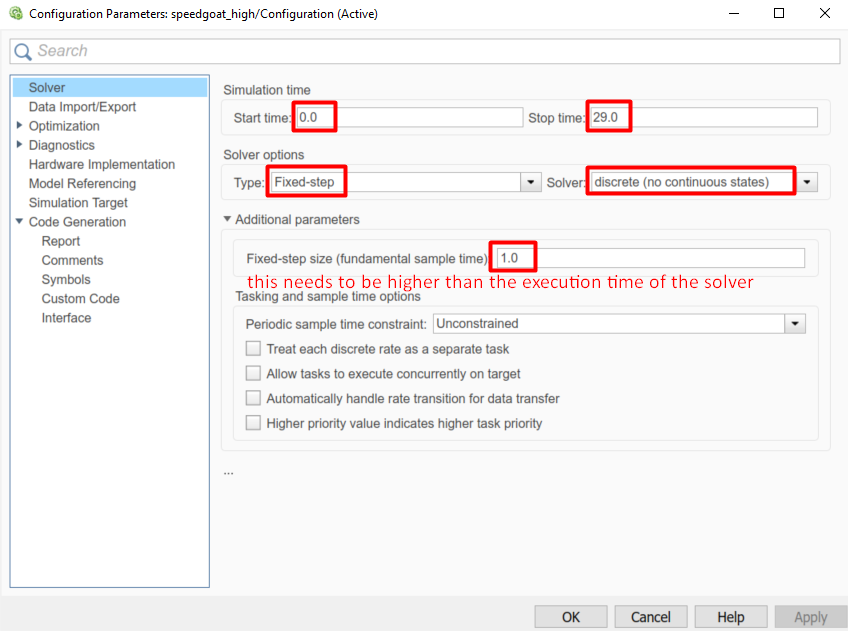
Figure 14.67 Set the Simulink solver options.
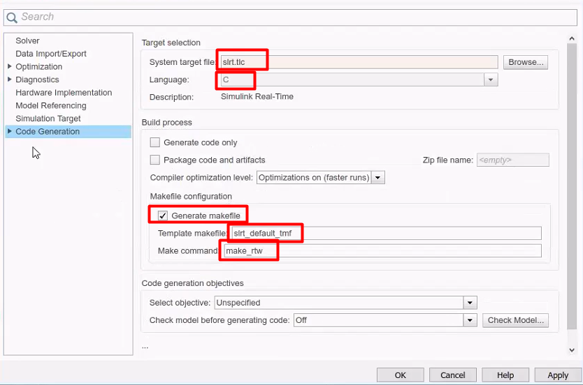
Figure 14.68 Set the Simulink code generation options.
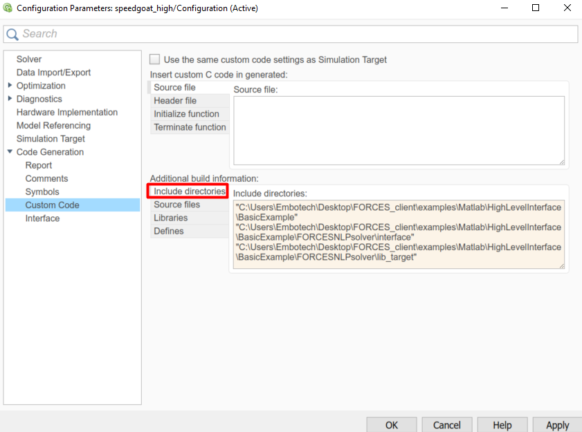
Figure 14.69 Add the directories included for the code generation.
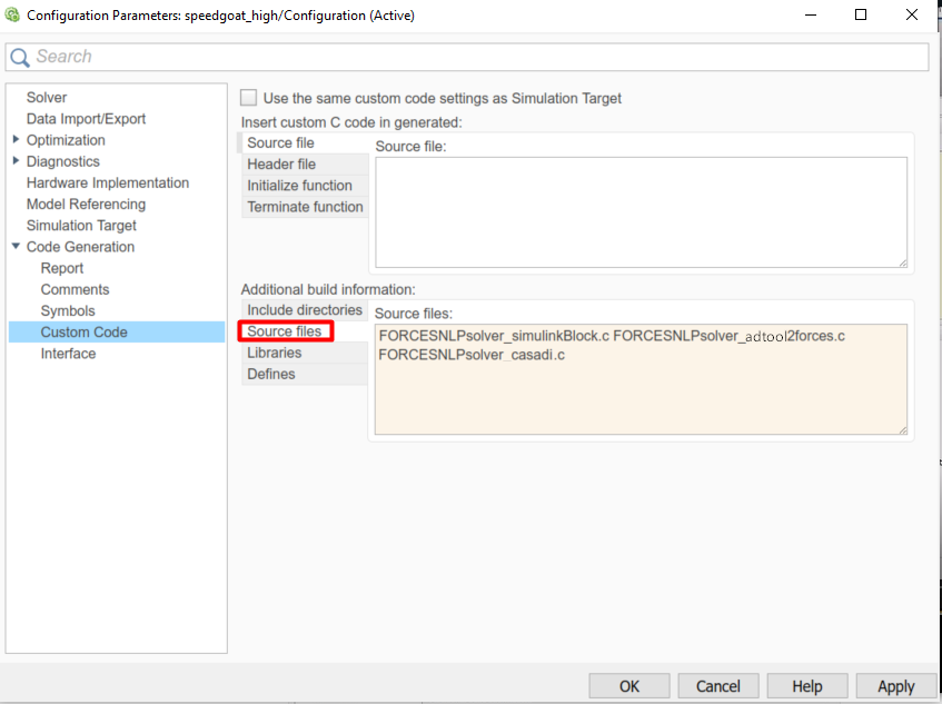
Figure 14.70 Add the source files used for the code generation.
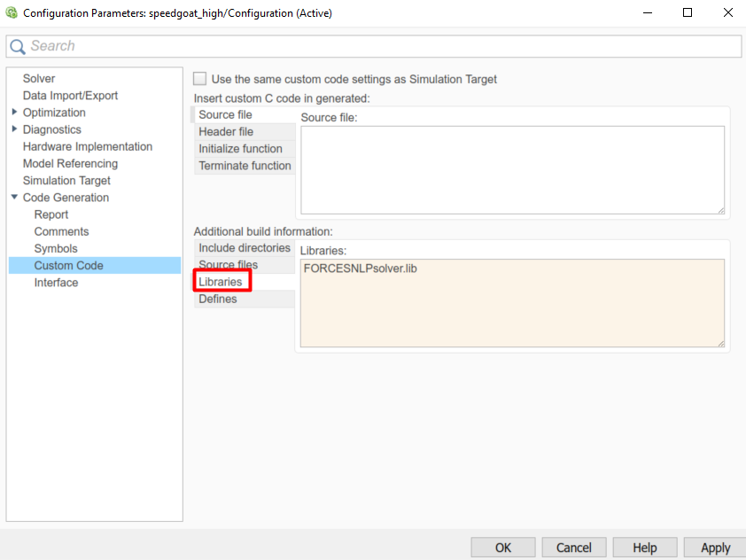
Figure 14.71 Add the libraries used for the code generation.
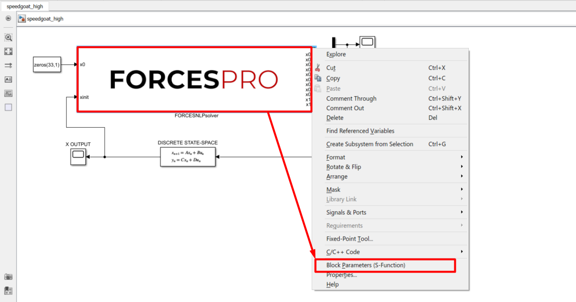
Figure 14.72 Open the FORCESPRO block’s parameters.
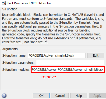
Figure 14.73 Remove the default data from the S-function module.
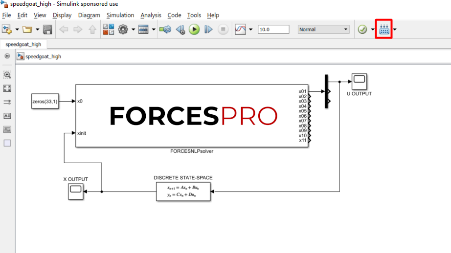
Figure 14.74 Compile the code of the Simulink model.
14.4.2. Y2F interface
14.4.2.1. Instructions
The steps to deploy and simulate a FORCESPRO controller on a Speedgoat platform are detailed below.
(Figure 14.75) Set the code generation options:
codeoptions.platform = 'Speedgoat-x86'; % to specify the platform
codeoptions.printlevel = 0; % on some platforms printing is not supported
and then generate the code for your solver (henceforth referred to as “simplempc_solver”, placed in the folder “Y2F”) using the Y2F interface.
(Figure 14.76) Create a new Simulink model using the blank model template.
(Figure 14.77) Populate the Simulink model with the system you want to control.
(Figure 14.78) Make sure the
simplempc_solver_simulinkBlock.mexw64file (created during code generation) is on the MATLAB path.(Figure 14.79) Copy-paste the FORCESPRO Simulink block, contained in the created
y2f_simulink_lib.slxSimulink model file, into your simulation model and connect its inputs and outputs appropriately.(Figure 14.80) Access the Simulink model’s options.
(Figure 14.81) In the “Solver” tab, set the options:
Simulation start/stop time: Depending on the simulation wanted.
Solver type: Discrete or fixed-step.
Fixed-step size: Needs to be higher than the execution time of the solver.
(Figure 14.82) In the “Code Generation/RTI general build options” tab, set the options:
System target file:
slrt.tlcLanguage: C
Generate makefile: On
Template makefile:
slrt_default_tmfMake command:
make_rtw
(Figure 14.83) In the “Code Generation/Custom Code” tab, include the directories:
Y2F\simplempc_solver\interface
Y2F\simplempc_solver\lib_target
(Figure 14.84) In the “Code Generation/Custom Code” tab, add the source files:
simplempc_solver_simulinkBlock.c
simplempc_solver.c
(Figure 14.85) In the “Code Generation/Custom Code” tab, add the library files:
i_simplempc_solver_1.lib
(Figure 14.86) Compile the code of the Simulink model. This will also automatically load the model to the connected Speedgoat platform.
Deployment is complete and simulations can now be run on the Speedgoat platform.
Run the simulation on the Speedgoat platform.
You can download the MATLAB code of this simulation to try it out for yourself by clicking
here.
14.4.2.2. Figures
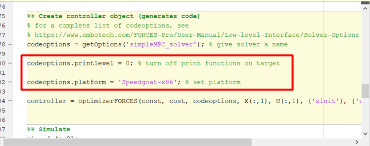
Figure 14.75 Set the appropriate code generation options.

Figure 14.76 Create a Simulink model.
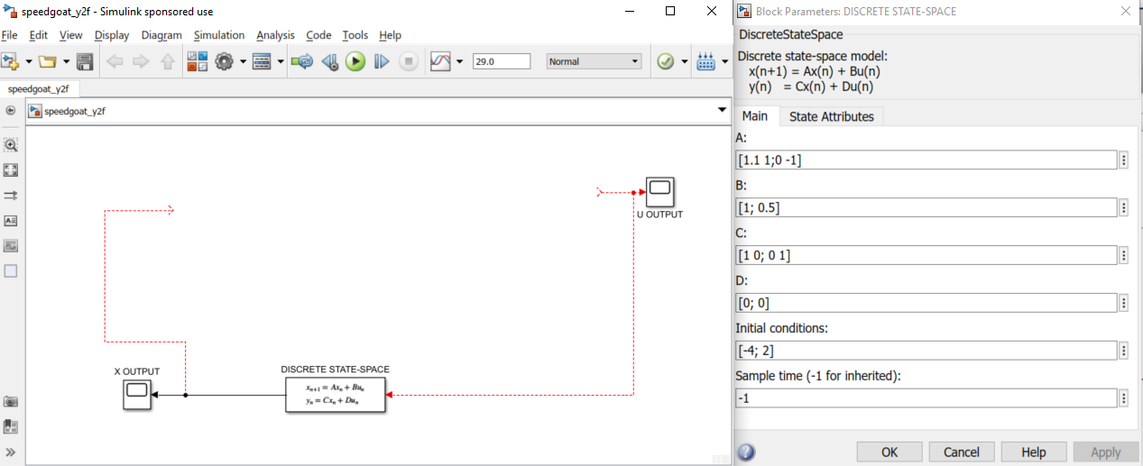
Figure 14.77 Populate the Simulink model.
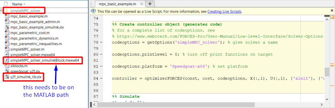
Figure 14.78 Add the folder containing the .mexw64 solver file to the MATLAB path.
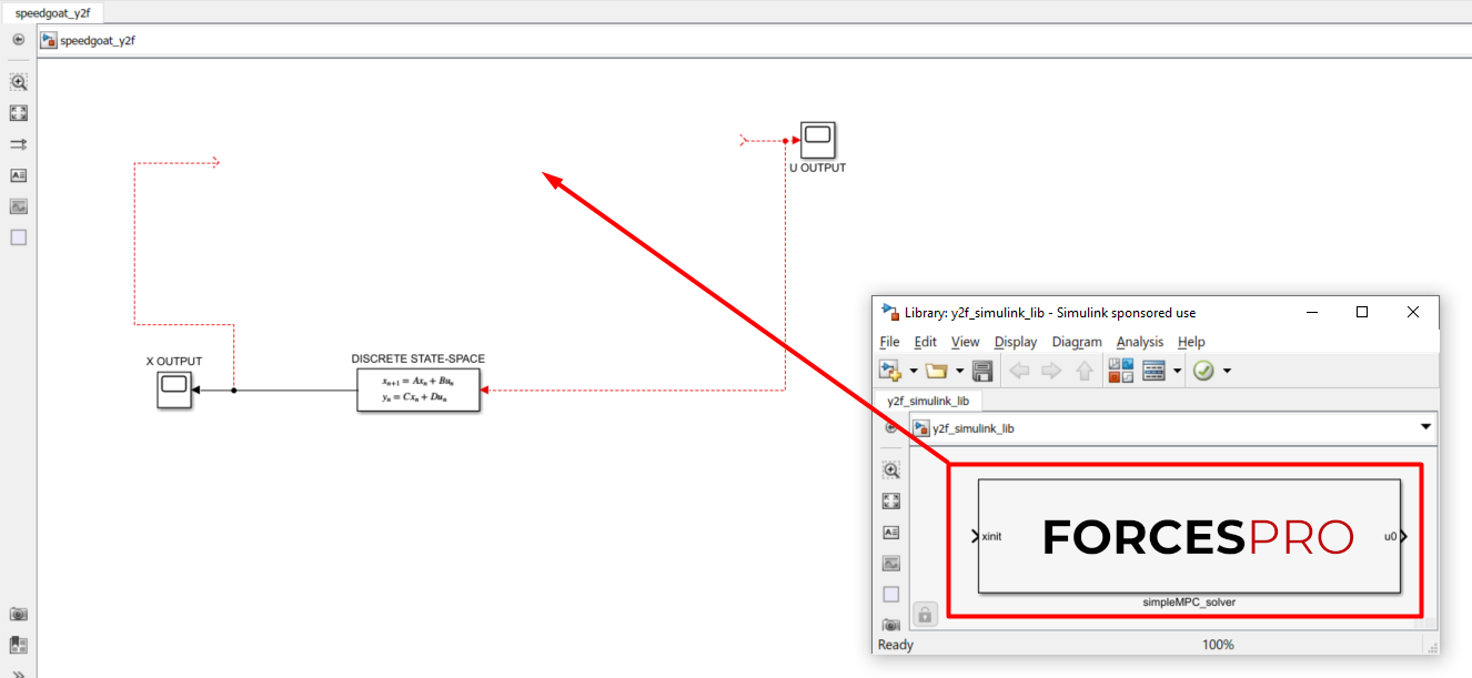
Figure 14.79 Copy-paste and connect the FORCESPRO block.
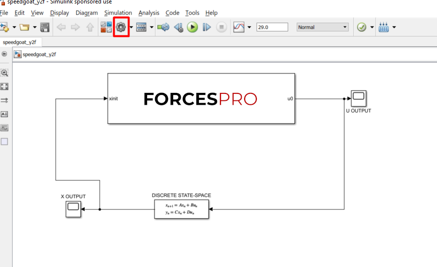
Figure 14.80 Open the Simulink model options.
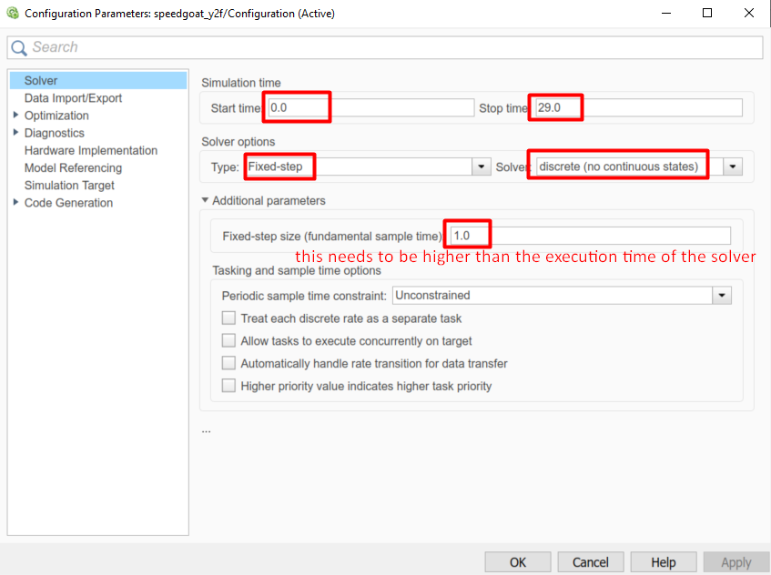
Figure 14.81 Set the Simulink solver options.
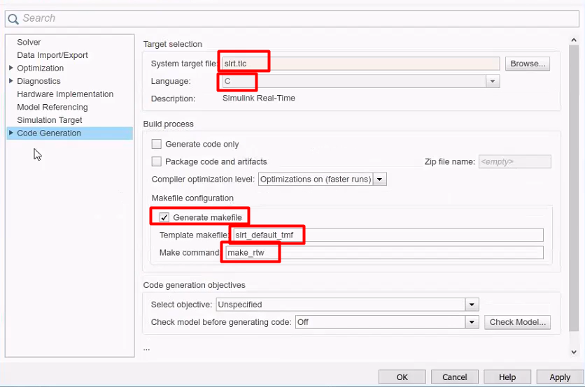
Figure 14.82 Set the Simulink code generation options.
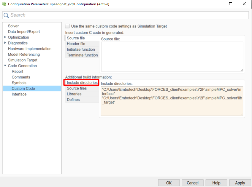
Figure 14.83 Add the directories included for the code generation.
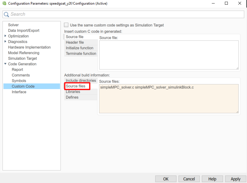
Figure 14.84 Add the source files used for the code generation.
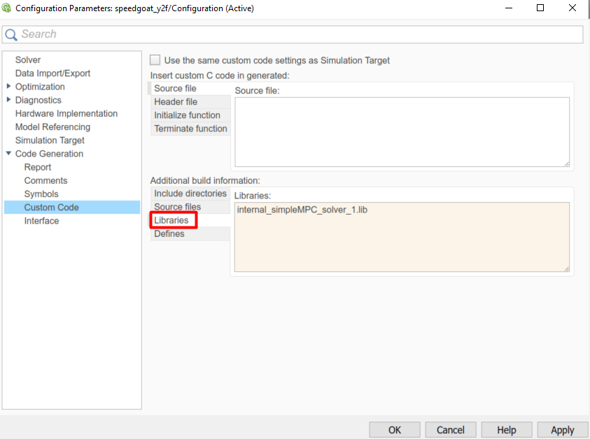
Figure 14.85 Add the libraries used for the code generation.
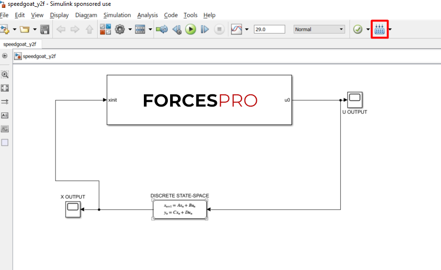
Figure 14.86 Compile the code of the Simulink model.