11.17. Controlling a DC motor using a FORCESPRO SQP solver
In this example our aim is to control a DC-motor using a FORCESPRO SQP solver. The model for the DC motor which we consider is borrowed from [BerUnb], to which we refer for further details. The dynamics of our model is described by the following set of ordinary differential equations:
The states \(x_1\) and \(x_2\) model the armature current and motor angular speed of out DC motor respectively and the control \(u\) models the input field current. The following values are chosen for our model constants
The control objective is to track a piecewise constant angular speed. To test the robustness of out resulting controller we switch reference half way through our simulation. In the first half of the simulation we will track a constant angular speed \(x_2^{ref1} = 2\) and then switch to tracking a constant angular speed \(x_2^{ref2} = -2\). We collect the 2-dimensional state vector \(x = (x_1, x_2)^T\) and the 1-dimensional control \(u\) in the vector
You can download the following MATLAB code of this example to try it out for yourself
by clicking here.
11.17.1. Defining the MPC problem
11.17.1.1. The tracking objective function
Since we want to track a reference value it is natural to consider a least squared cost \(f(z,p) = \frac{|\!| r(z,p) |\!|^2}{2}\) for
Recall that \(z_3=x_2\) models the motor angular speed which is made to track a piecewise constant reference. The parameter \(p\) will be equal to \(x_2^{ref1}\) during the first half of the simulation and equal to \(x_2^{ref2}\) during the second.
The following code snippet reads in the least squared objective
model.LSobjective = @(z,p) sqrt(100) * (z(3) - p);
model.LSobjectiveN = @(z,p) sqrt(100) * (z(3) - p);
11.17.1.2. The dynamics
The following code snippet reads in the dynamics (11.1) of our model:
%% model parameters
% Armature inductance (H)
La = 0.307;
% Armature resistance (Ohms)
Ra = 12.548;
% Motor constant (Nm/A^2)
km = 0.23576;
% Total moment of inertia (Nm.sec^2)
J = 0.00385;
% Total viscous damping (Nm.sec)
B = 0.00783;
% Load torque (Nm)
tauL = 1.47;
% Armature voltage (V)
ua = 60;

model.E = [zeros(2,1), eye(2)];
model.continuous_dynamics = @(x,u) [(-1/La)*(Ra*x(1) + x(2)*u(1) - ua); ...
                                           (-1/J)*(B*x(2) - km*x(1)*u(1) + tauL)];
11.17.1.3. Input and state constraints
The following constraints are to be met by out control and state vectors:
This can be read into the FORCESPRO model as follows
model.lb = [1; -5; -10];
model.ub = [1.6; 5; 2.004];
11.17.1.4. Generating the FORCESPRO SQP solver
To generate a suitable SQP solver for out MPC problem one need a model struct as well as a codeoptions struct. Our model struct has been
populated above and we now specify the codeoptions we want and generating the solver by calling FORCES_NLP. The following code-snippet shows how this can be done:
%% set codeoptions
codeoptions = getOptions('FORCESPROSolver');
codeoptions.solvemethod = 'SQP_NLP'; % generate SQP-RTI solver
codeoptions.nlp.ad_tool = 'casadi';
codeoptions.BuildSimulinkBlock = 0;
codeoptions.nlp.integrator.type = 'ERK4';
integration_step = 0.01;
codeoptions.nlp.integrator.Ts = integration_step;
codeoptions.nlp.integrator.nodes = 1;
codeoptions.nlp.hessian_approximation = 'gauss-newton';
codeoptions.timing = 1;

%% generate FORCESPRO solver
FORCES_NLP(model, codeoptions);
11.17.1.5. Calling the solver
Once the solver has been generated it needs a struct containing an initial guess, initial condition of the ODE, the run-time parameters and the reinitialize
field as explained in Sequential quadratic programming algorithm. The following code-snippet shows how this can be done:
% populate run time parameters struct
params.all_parameters = repmat(2, model.N, 1);
params.xinit = zeros(model.neq, 1); % initial condition to ODE
params.x0 = repmat([1.2; zeros(2,1)], model.N, 1); % initial guess
params.reinitialize = 0;

% Solve optimization problem
[output, exitflag, info] = FORCESPROSolver(params);
The FORCESPROSolver is expected to return an exitflag equal to \(1\), which corresponds to a
successful solve. However, note that the QP could become infeasible in some cases. In this
case, one should expect an exitflag equal to \(−8\).
11.17.1.6. Results
The control objective is to track an angular speed of 2 and -2 respectively. As can be seen in Figure 11.57 the controller completes this task. The control (\(u\)) is plotted in Figure 11.53, the first state (\(x_1\)) is plotted in Figure 11.54 and second state (\(x_2\)) in Figure 11.55. As a measure of control quality, the closed loop objective value is plotted in Figure 11.56.
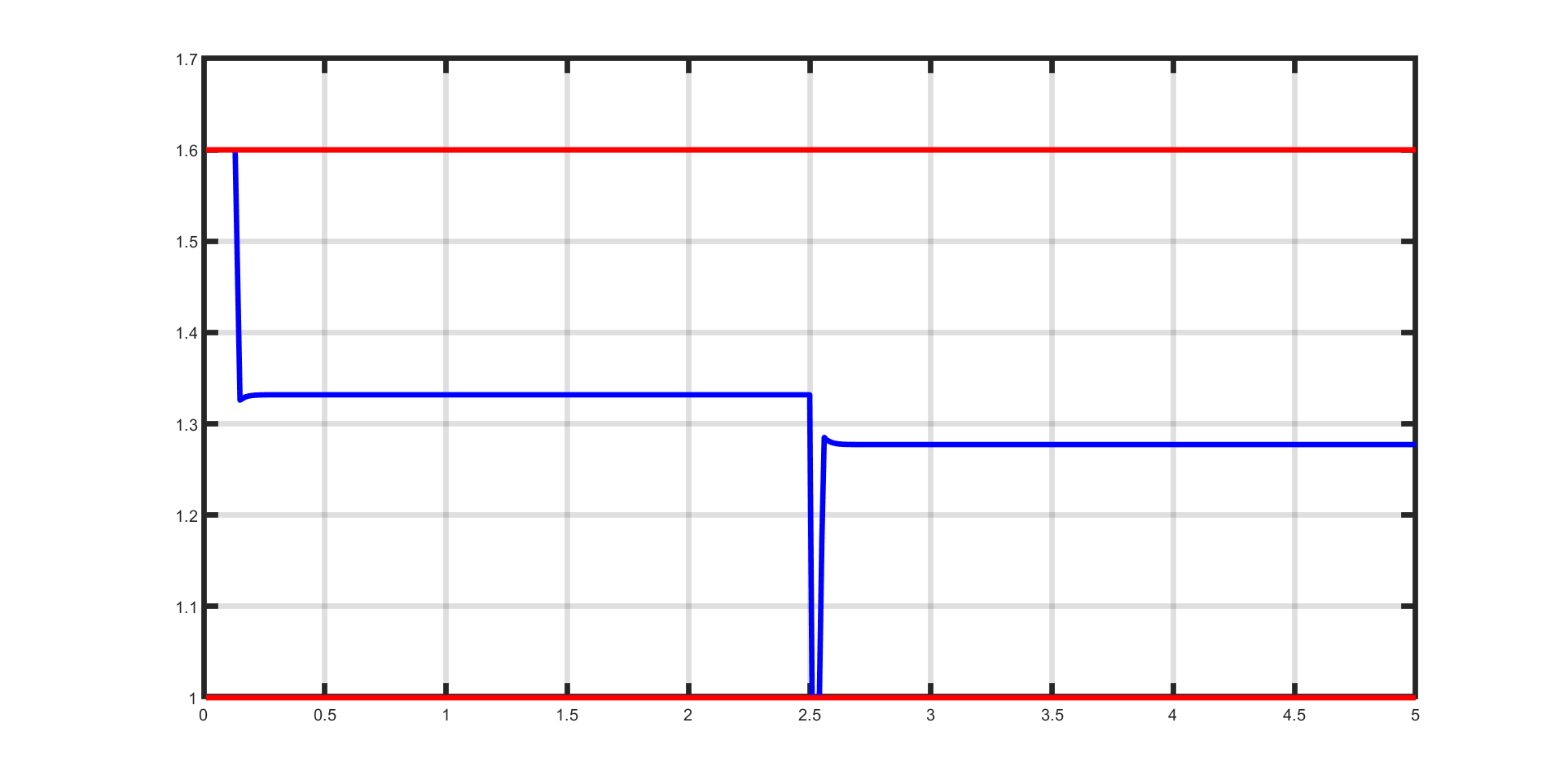
Figure 11.53 The control (\(u\), in blue) as a function of simulation time (s). The control obeys its constraints (red) throughout the simulation.
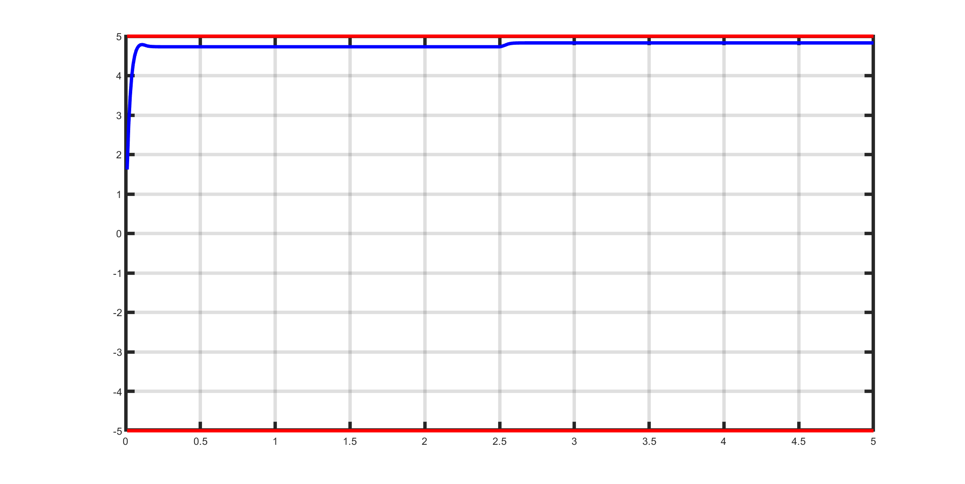
Figure 11.54 The first state (\(x_1\), in blue) as a function of simulation time. It obeys its constraints (red) throughout the simulation.
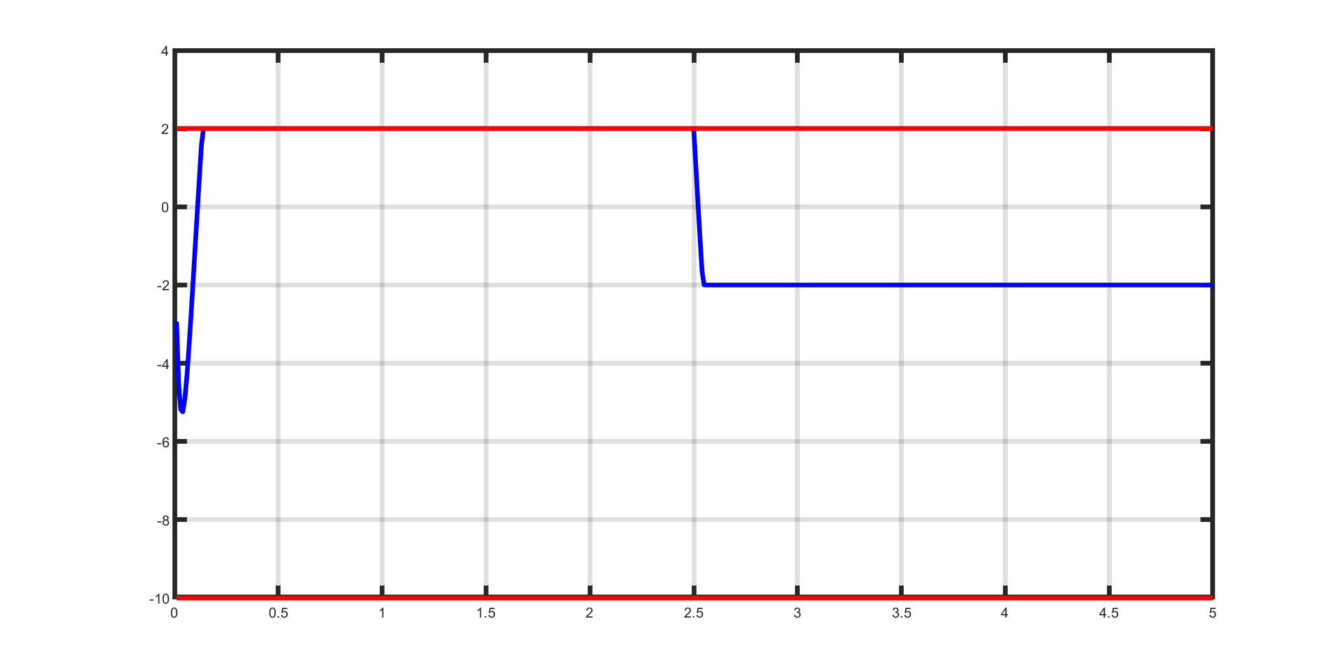
Figure 11.55 The second state (\(x_2\), in blue) as a function of simulation time. It obeys its constraints (red) throughout the simulation.
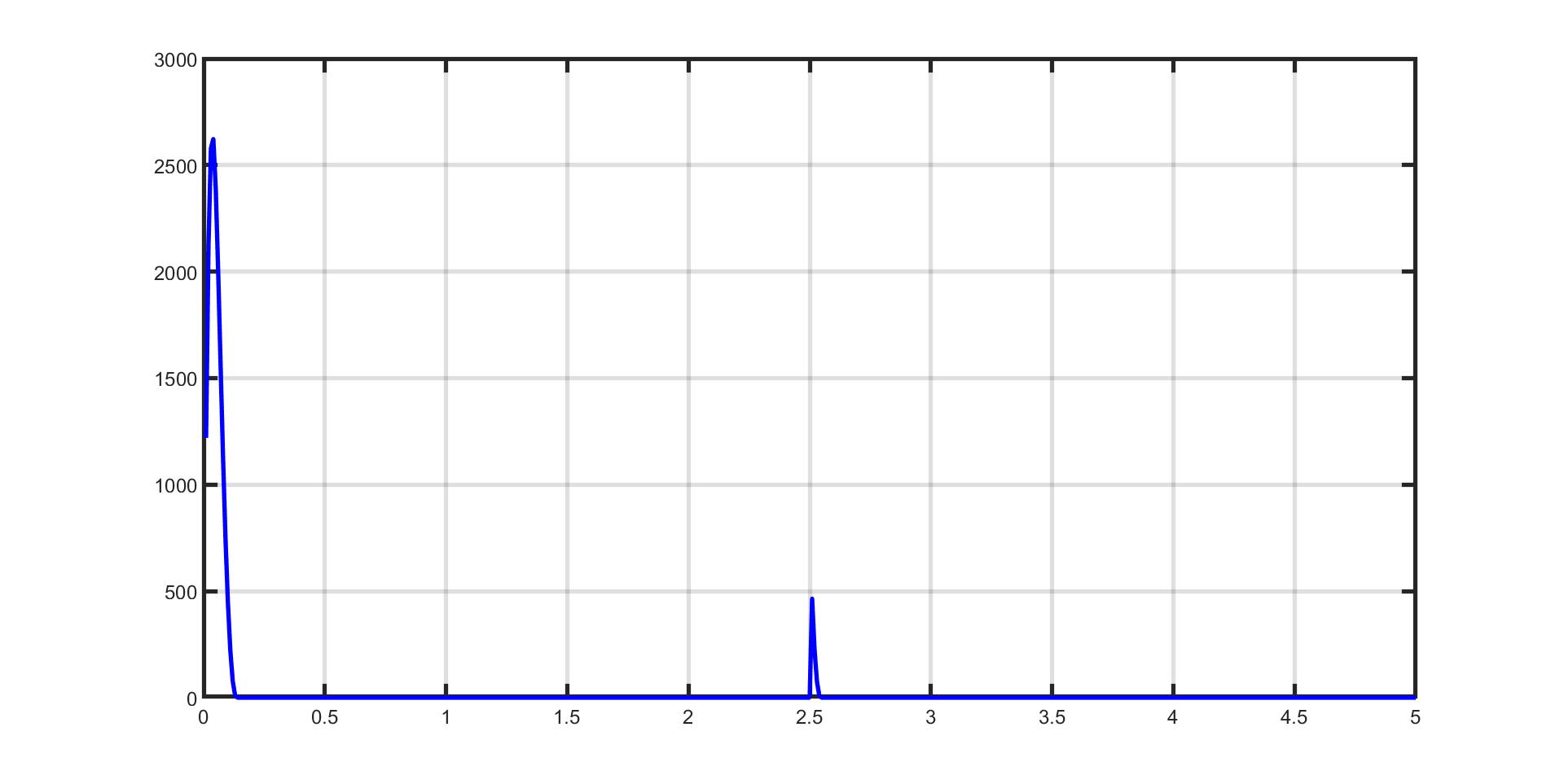
Figure 11.56 Closed-loop objective value as a function of time
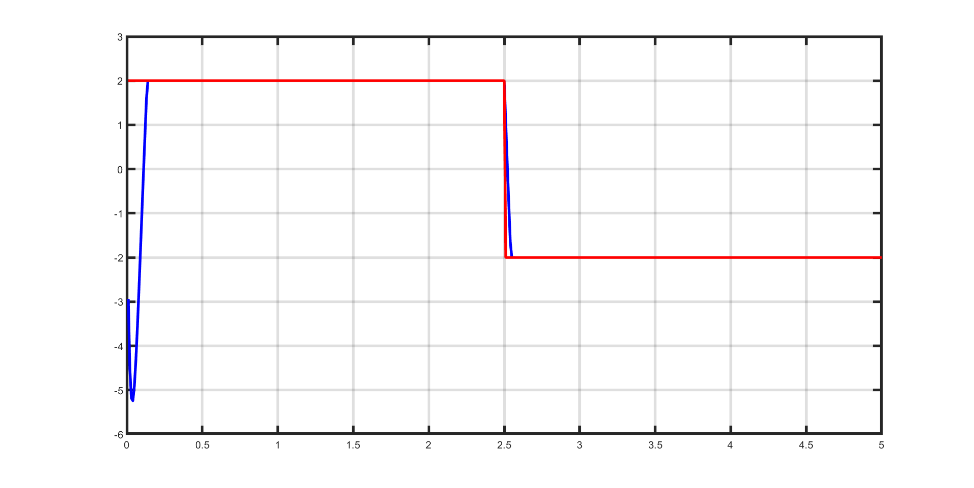
Figure 11.57 Angular speed (blue) and tracked reference (red) value as a function of time.
S. Daniel-Berhe; H. Unbehauen: Experimental physical parameter estimation of a thyristor driven DC-motor using the HMF-method. Control Engineering Practice, 6:615–626, 1998