11.9. High-level interface: Obstacle avoidance (MATLAB & Python)

In this example we illustrate the simplicity of the high-level user interface on a vehicle optimal trajectory generation problem. The user can place an obstacle in front of the vehicle using an interactive window and the car trajectory is automatically adjusted.

In particular, we use a kinematic bicycle model described by a set of ordinary differential equations (ODEs):

\[\begin{split}\dot{x} & = v \cos(\theta + \beta) \\ \dot{y} & = v \sin(\theta + \beta) \\ \dot{v} & = \frac{F}{m} \\ \dot{\theta} & = \frac{v}{l_r} \sin(\beta) \\ \dot{\delta} &= \phi\end{split}\]

with:

\[\beta = \arctan( \frac{l_r}{l_r + l_f} \tan( \delta))\]

The model consists of five differential states: \(x\) and \(y\) are the Cartesian coordinates of the car, and \(v\) is the linear velocity. The angles \(\theta\) and \(\delta\) denote the heading angle of the car and its steering angle. Next, there are two control inputs to the model: the acceleration force \(F\) and the steering rate \(\phi\). The angle \(\beta\) describes the direction of movement of the car’s center of gravity relative to the heading angle \(\theta\). The remaining three constant parameters of the system are the car mass \(m=1\,\mathrm{kg}\), and the lengths \(l_r=0.5\,\mathrm{m}\) and \(l_f=0.5\,\mathrm{m}\) specifying the distance from the car’s center of gravity to the rear wheels and the front wheels, respectively.

The trajectory of the vehicle will be defined as an NLP. First, we define stage variable \(z\) by stacking the input and differential state variables:

\[z = [F,\phi,x,y,v,\theta,\delta]^\top\]

You can download the code of this example to try it out for yourself by clicking here (MATLAB) or here (Python).

11.9.1. Defining the MPC Problem

11.9.1.1. Objective

In this example the cost function provided by model.objective is the same for all stages. We have a target position \((3,0)\) and we want to minimize the distance of the car to that point. Therefore, the distance is penalized with linear costs. Plus, some small quadratic costs are added to the inputs \(F\) and \(s\), i.e.:

\[f(z) = 100 |z_3 - 0| + 100 |z_4 - 3| + 0.1 z_1^2 + 0.01 z_2^2\]

The stage cost function is coded in MATLAB and Python as the following function:

MatlabPython

model.objective = @objective

function f = objective(z)
    F = z(1);
    phi = z(2);
    x = z(3)
    y = z(4);
    f = 100*abs(x-0) + 100*abs(y-3) + 0.1*F^2 + 0.01*phi^2;
end

11.9.1.2. Matrix equality constraints

The matrix equality constraints model.eq in this example result from the vehicle’s dynamics given above. First, the continuous dynamic equations are implemented as follows:

MatlabPython

function [xDot] = continuousDynamics(x,u)
  % state x = [xPos,yPos,v,theta,delta], input u = [F, phi]

      % set physical constants
      l_r = 0.5; % distance rear wheels to center of gravity of the car
      l_f = 0.5; % distance front wheels to center of gravity of the car
      m = 1.0;   % mass of the car

      % set parameters
      beta = atan(l_r/(l_f + l_r) * tan(x(5)));

      % calculate dx/dt
      xDot = [x(3) * cos(x(4) + beta); % dxPos/dt = v*cos(theta+beta)
              x(3) * sin(x(4) + beta); % dyPos/dt = v*cos(theta+beta)
              u(1)/m;                  % dv/dt = F/m
              x(3)/l_r * sin(beta);    % dtheta/dt = v/l_r*sin(beta)
              u(2)];                   % ddelta/dt = phi
  end

Now, these continuous dynamics are discretized using an explicit Runge-Kutta integrator of order 4 as shown below. Note that the function RK4 is included in the FORCESPRO client software.

MatlabPython

integrator_stepsize = 0.1;
% z(3:7) = states x, z(1:2) = inputs u
model.eq = @(z) RK4(z(3:7), z(1:2), @continuousDynamics, integrator_stepsize);

As a last step, the indices of the left hand side of the dynamical constraint are defined. For efficiency reasons, make sure the matrix has structure [0 I].

MatlabPython

model.E = [zeros(5,2), eye(5)];

11.9.1.3. Runtime Parameters

The user can place an obstacle to be avoided in front of the car. The x- and y-coordinates of the position \(p\) of this obstacle are considered as runtime parameters of the system.

\[p = [p_x,p_y]^\top\]

The runtime parameters are the same for all stages. Their values will be set later on at runtime.

11.9.1.4. Inequality constraints

The maneuver is subjected to a set of constraints, involving both the simple bounds:

\begin{align*} -5\,\mathrm{N} \leq & F \leq 5\,\mathrm{N} \\ -40\,\mathrm{deg/s} \leq & \phi \leq 40\,\mathrm{deg/s} \\ -3\,\mathrm{m} \leq & x \leq 0\,\mathrm{m} \\ 0\,\mathrm{m} \leq & y \leq 3\,\mathrm{m} \\ 0\,\mathrm{m/s} \leq & v \leq 2\,\mathrm{m/s} \\ -\inf \leq & \theta \leq \inf \\ -0.48 \pi\,\mathrm{rad} \leq & \delta \leq 0.48 \pi\,\mathrm{rad} \\ \end{align*}

as well the nonlinear nonconvex constraints in dependence of the runtime parameters \(p\)

\begin{align*} 1\,\mathrm{m^2} \leq & x^2+y^2 \leq 9\,\mathrm{m^2} \\ 0.7^2\,\mathrm{m^2} \leq & (x-p_x)^2 + (y-p_y)^2 \\ \end{align*}

The implementation of the simple bounds is given here:

MatlabPython

% upper/lower variable bounds lb <= z <= ub
%            inputs             |             states
%             F      phi            x     y     v    theta    delta
model.lb = [ -5.0,  deg2rad(-40),  -3.,   0.,   0.,  -inf,   -0.48*pi];
model.ub = [ +5.0,  deg2rad(+40),   0.,   3.,   2.,  +inf,    0.48*pi];

The nonlinear constraint function \(h\) with its bounds can be coded in MATLAB/Python as follows:

MatlabPython

% General (differentiable) nonlinear inequalities hl <= h(x,p) <= hu
model.ineq = @(z,p)  [   z(3)^2 + z(4)^2;                 % x^2 + y^2
                        (z(3)-p(1))^2 + (z(4)-p(2))^2 ];  % (x-p_x)^2 + (y-p_y)^2

 % Upper/lower bounds for inequalities
model.hu = [9, +inf]';
model.hl = [1, 0.7^2]';

11.9.1.5. Dimensions

Furthermore, the number of variables, constraints and real-time parameters explained above needs to be provided as well as the length of the multistage problem. For this example, we chose to use \(N = 50\) stages in the NLP:

MatlabPython

model.N = 50;    % horizon length
model.nvar = 7;  % number of variables
model.neq  = 5;  % number of equality constraints
model.nh = 2;    % number of inequality constraint functions
model.npar = 2;  % number of runtime parameters
model.bfgs_init = 3.0*eye(7);  % set initialization of the hessian approximation

11.9.1.6. Initial conditions

The goal of the maneuver is to steer the vehicle from a set of initial conditions:

\[x_{\mathrm{init}} = -2\,\mathrm{m} ,\quad y_{\mathrm{init}} = 0\,\mathrm{m} ,\quad v_{\mathrm{init}} = 0\,\mathrm{m/s} ,\quad \theta_{\mathrm{init}} = 0.5 \pi\,\mathrm{rad}, ,\quad \delta_{\mathrm{init}} = 0\,\mathrm{rad}\]

For the code generation, only the indices of the variables to which initial values will be applied are required. This is coded as follows:

MatlabPython

model.xinitidx = 3:7;

11.9.2. Generating a solver

We have now populated model with the necessary fields to generate a solver for our problem. Now we set some options for our solver and then use the function FORCES_NLP to generate a solver for the problem defined by model:

MatlabPython

%% Define solver options
codeoptions = getOptions('FORCESNLPsolver');
codeoptions.maxit = 400;                 % Maximum number of iterations
codeoptions.printlevel = 0;
codeoptions.optlevel = 0;                % 0: no optimization, 1: optimize for size, 2: optimize for speed, 3: optimize for size & speed
codeoptions.printlevel = 0;

%% Generate forces solver
FORCES_NLP(model, codeoptions);

11.9.3. Calling the generated solver

Once all parameters of the problem instance to be solved have been populated, the MEX interface of the solver can be used to invoke it.

MatlabPython

% Set initial guess to start solver from (here, middle of upper and lower bound)
x0i=[0.0,0.0,-1.5,1.5,1.,pi/4.,0.];
x0=repmat(x0i',model.N,1);
problem.x0=x0;

% Set initial condition
problem.xinit = [-2., 0., 0., deg2rad(90), 0.]';

% Set runtime parameters
params = [-1.5; 1.0]; # In this example, the user can change these parameters by clicking into an interactive window
problem.all_parameters = repmat(params,model.N,1);

% Time to solve the NLP!
[output,exitflag,info] = FORCESNLPsolver(problem);

% Make sure the solver has exited properly.
assert(exitflag == 1,'Some problem in FORCES solver');
fprintf('\nFORCES took %d iterations and %f seconds to solve the problem.\n',info.it,info.solvetime);

11.9.4. Results

The goal is to find a trajectory that steers the vehicle from point A as close as possible to point B while avoiding obstacles. The trajectory should also be feasible with respect to the vehicle dynamics and its safety and physical limitations. The calculated vehicle’s trajectory in 2D space is presented in Figure 11.33. The progress of the other states and the inputs over time is shown in Figure 11.34. One can see that all constraints are respected. To try out other obstacle positions you can run the example file on your own machine and click into the interactive window.

You can download the code of this example by clicking here (MATLAB) or here (Python).

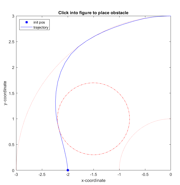
Figure 11.33 The calculated trajectory of the car

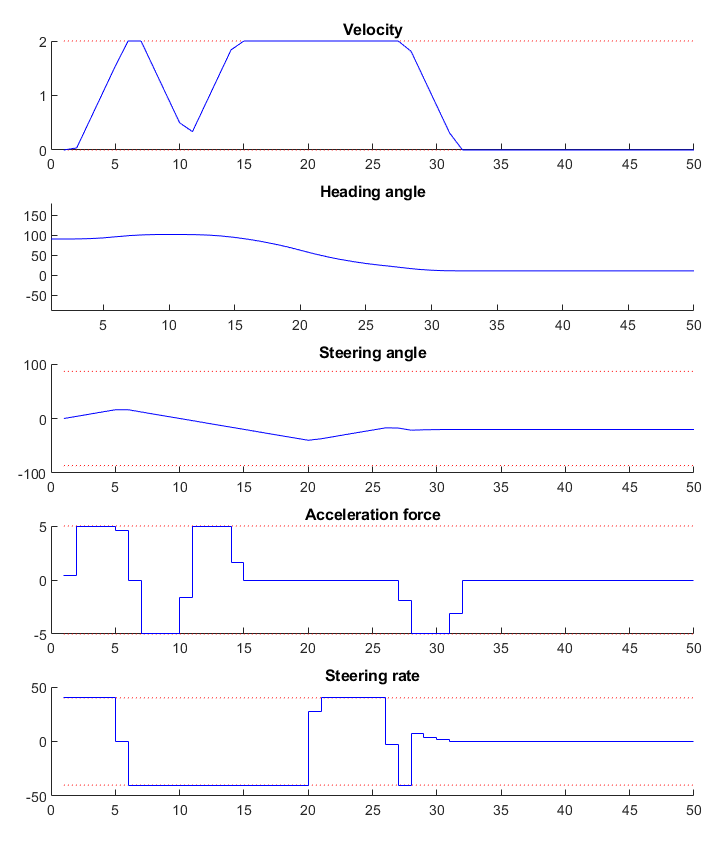
Figure 11.34 Development of the vehicle’s states and the system’s inputs over time

11.9.5. Variation: External functions

In this variation, we want to supply the required functions through external functions in C. To do so we have to provide the directory that contains said source files in the MATLAB code:

%% Define source file containing function evaluation code
model.extfuncs = 'C/myfevals.c';

We also need to include the two extern functions car_dynamics and car_dynamics_jacobian, both contained in the car_dynamics.c file, through the other_srcs options field:

% add additional source files required - separate by spaces if more than 1
codeoptions.nlp.other_srcs = 'C/car_dynamics.c';

In Python, we need to switch to an ExternalFunctionModel if we intend to use external callbacks. We give the main callback evaluating the objective function, equality constraints and inequality constraints, using the set_main_function() , and supply any additional files required by this callback using add_auxiliary().

model = forcespro.nlp.ExternalFunctionModel()

# Define source file containing function evaluation code
model.set_main_callback("C/myfevals.c", function="myfevals")
model.add_auxiliary("C/car_dynamics.c")
# One can also add a 'relative_to' argument specifying the paths to be understood
# relative to this file's location. if not supplied, paths are relative to the
# current working directory in which this script is executed:
# model.set_main_callback('c/myfevals.c', function="myfevals" relative_to=os.path.dirname(__file__))
# model.add_auxiliary('c/car_dynamics.c', relative_to=os.path.dirname(__file__))

You can download the code of this variation to try it out for yourself by clicking here (MATLAB) or here (Python). The C-code for the function evaluations and the car dynamics is also available.