11.1.6. Binary MPC Example

Let us consider a simple MPC example where the system has inputs that can take only two values, \(u_{min}\) or \(u_{max}\). The original problem (shown on the left) can be reformulated into the problem on the right, which corresponds to a standard form for which FORCESPRO can generate a solver. The details of the reformulation are given at the end of this example.

Simple MPC problem with discrete inputs:

\begin{align*} \text{minimize} \quad & x_N^T P x_N + \sum_{i=0}^{N-1}x_i^T Q x_i + u_i^T R u_i \\ \text{subject to} \quad & x_0 = x \\ & x_{i+1}=Ax_i + Bu_i \\ & x_{min}\leq x_i \leq x_{max} \\ & u_i \in \{ u_{min}, u_{max} \} \end{align*}

Equivalent problem with binary inputs

\begin{align*} \text{minimize} \quad & x_N^T P x_N + \sum_{i=0}^{N-1}x_i^T Q x_i + \delta_i^T \tilde{R}\delta_i + \tilde{f}^T \delta_i \\ \text{subject to} \quad & x_0 = x \\ & x_{i+1}=Ax_i + \tilde{B}\delta_i + b \\ & x_{min}\leq x_i \leq x_{max} \\ & \delta_i \in \{ 0,1 \}^{n_u} \end{align*}

The problem on the right can now be easily formulated in FORCESPRO. Note that the problem description is very similar to that of the simple MPC example, with the only modification that certain variables are marked to be binary. Download and run a complete simulation script to see the output.

nx = 2; nu = 2;

% assume variable ordering zi = [delta_{i-1}; x{i}] for i=1...N
stages = MultistageProblem(N);
for i = 1:N
  % dimension
  stages(i).dims.n = nx+nu; % number of stage variables
  stages(i).dims.r = nx; % number of equality constraints
  stages(i).dims.l = nx; % number of lower bounds
  stages(i).dims.u = nx; % number of upper bounds
  stages(i).bidx = 1:nu; % index of binary variables

  % cost
  if( i == N )
        stages(i).cost.H = blkdiag(Rtilde,P);
  else
        stages(i).cost.H = blkdiag(Rtilde,Q);
  end
  stages(i).cost.f = [ftilde; zeros(nx,1)];

  % lower bounds
  stages(i).ineq.b.lbidx = (nu+1):(nu+nx); % lower bound on states
  stages(i).ineq.b.lb = xmin; % upper bound values

  % upper bounds
  stages(i).ineq.b.ubidx = (nu+1):(nu+nx); % upper bound for this stage variable
  stages(i).ineq.b.ub = umax; % upper bound for this stage variable

  % equality constraints
  if( i < N )
        stages(i).eq.C = [zeros(nx,nu), A];
  end
  if( i>1 )
        stages(i).eq.c = -Bconst;
  end
  stages(i).eq.D = [Btilde, -eye(nx)];
end

% RHS of first eq. constr. is a parameter: z1=-A*x0
params(1) = newParam('minusA_times_x0',1,'eq.c');

You can download the MATLAB code of this example to try it out for yourself by clicking here.

You can download the Python code of this example to try it out for yourself by clicking here.

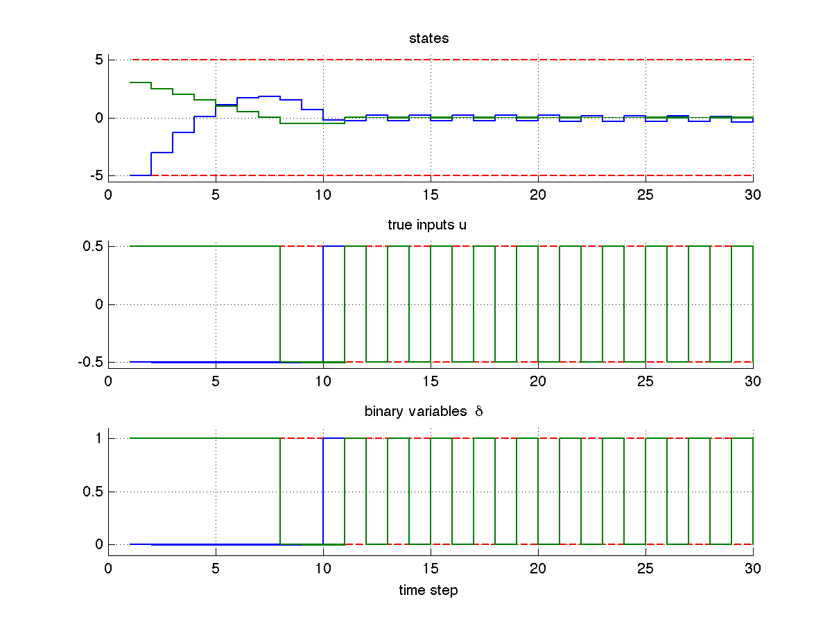
11.1.6.1. Simulation result

When running the example, you should see the following closed-loop behavior:

11.1.6.2. Details on problem reformulation

The reformulation is done as follows: we introduce a variable \(delta\) such that

\[\delta = 0 \Leftrightarrow u=u_{min} \quad \text{and} \quad \delta = 0 \Leftrightarrow u = u_{max}\]

This can be formulated by the equality constraint

\[u = u_{min} + \text{diag}(u_{max} - u_{min})\delta\]

where \(\text{diag}\) denotes a diagonal matrix. To keep the number of variables at a minimum, we will directly insert this equation into the dynamics:

\begin{align*} x^+ &= Ax + Bu \\ &= Ax + Bu_{min} + B \text{diag}(u_{max}- u_{min})\delta \\ &= Ax + \tilde{B}\delta + b \end{align*}

where \(\tilde{B}:=B \text{diag}(u_{max}-u_{min})\) and \(b:=B u_{min}\).

Similarly for the cost function,

\begin{align*} u^T R u &= (u_{min} + \text{diag}(u_{max}-u_{min})\delta )^T R (u_{min} + \text{diag}(u_{max}-u_{min})\delta ) \\ &= \delta^T \text{diag}(u_{max}-u_{min}) R \text{diag}(u_{max}-u_{min}) \delta + 2 u_{min} \text{diag}(u_{max}-u_{min})R \delta + \text{const} \\ &= \delta^T \tilde{R} \delta + \tilde{f}^T \delta + \text{const} \end{align*}

where

\[\begin{split}\tilde{R} & = \text{diag}(u_{max}-u_{min}) R \text{diag}(u_{max}-u_{min}) \\ \tilde{f} & = 2R \text{diag}(u_{max}-u_{min})u_{min}\end{split}\]