11.1.5. HOW TO: Implement Rate Constraints

11.1.5.1. Problem formulation

In this example it is illustrated how slew rate constraints on a system’s actuators can be incorporated in the controller design. As a real world example one could think of an airplane, where the elevator cannot be switched instantaneously from one position to another, i. e. has a limited slew rate. Here the concept of constraints on the slew rate is shown on the following system:

\begin{align*} x_{k+1}= \begin{pmatrix} 0.7115 & -0.4345 \\ 0.4345 & 0.8853 \end{pmatrix} x_k + \begin{pmatrix} 0.2173 \\ 0.0573 \end{pmatrix}u_k \Leftrightarrow x_{k+1}=Ax_k +Bu_k \end{align*}

To have a bound on the slew rate, \(u_k − u_{k−1}\) has to lie in some range, i. e.

\[\Delta u_{min} \leq u_k−u_{k−1} \leq \Delta u_{max}.\]

One option to set the constraints on the slew rate is to augment the state as follows:

\[\begin{split}\hat{x}_{k}= \begin{pmatrix} x_k \\ u_{k-1} \end{pmatrix} \quad \Leftrightarrow \quad \hat{x}_{k+1}= \begin{pmatrix} A & B \\ 0 & I \end{pmatrix}\hat{x}_k + \begin{pmatrix} B \\ I \end{pmatrix}\hat{u}_k \quad \Leftrightarrow \quad \hat{x}_{k+1}= \hat{A} \hat{x}_k + \hat{B}\hat{u}_k\end{split}\]

where \(\hat{u}\) is defined as \(u_k − u_{k−1}\). To implement the problem using FORCESPRO, the multistage problem has to be defined as stated here. The optimization variable is \(z_i = [ \hat{u}_i \quad \hat{x}_{i+1}]^T\).

\begin{align*} \hat{x}_{k+1}=& \hat{A} \hat{x}_k + \hat{B}\hat{u}_k \\ \Delta u_{min} &\leq \hat{u} \leq \Delta u_{max} \\ u_{min} \leq& u \leq \Delta u_{max} \\ &\Big\Downarrow \\ \text{minimize}& \quad \frac{1}{2}\sum_{i=1}^{N} z_i^T H_i z_i \\ \text{subject to}& \quad D_1 z_1 = c_1 \\ & \quad C_{i-1}z_{i-1} + D_{i}z_i = c_i \\ & \quad z_{min} \leq z_i \leq z_{max} \end{align*}

The details on how the first equality and the interstage equality look like and how the constraints are implemented can be seen in the MATLAB® code below.

11.1.5.2. Implementation

%% FORCES multistage form
% assume variable ordering zi = [uhat_{i-1}, xhat_{i}] for i=1...N

stages = MultistageProblem(N); % get stages struct of length N

for i = 1:N

        % dimension
        stages(i).dims.n = 4; % number of stage variables
        stages(i).dims.r = 3; % number of equality constraints
        stages(i).dims.l = 2; % number of lower bounds: minimal slew rate and minimal input
        stages(i).dims.u = 2; % number of upper bounds: maximal slew rate and maximal input

        % cost
        if( i == N )
                stages(i).cost.H = blkdiag(R_sr, [P, zeros(2,1); zeros(1,2), 0]); % terminal cost (Hessian)
        else
                stages(i).cost.H = blkdiag(R_sr, [Q, zeros(2,1); zeros(1,2), R]);
        end
        stages(i).cost.f = zeros(3,1); % linear cost terms

        % lower bounds
        stages(i).ineq.b.lbidx = [1,4]; % indices of lower bounds
        stages(i).ineq.b.lb = [dumin; umin]; % lower bounds

        % upper bounds
        stages(i).ineq.b.ubidx = [1,4]; % indices of upper bounds
        stages(i).ineq.b.ub = [dumax; umax]; % upper bounds

        % equality constraints
        if( i < N )
                 stages(i).eq.C = [zeros(3,1), [ A, B; zeros(1, 2), 1]];
        end
        if( i>1 )
                 stages(i).eq.c = zeros(3,1);
        end
        stages(i).eq.D = [[B;1], -eye(3)];

end

% RHS of initial equality constraint is a parameter
parameter(1) = newParam('minusAhat_times_xhat0',1,'eq.c');

% Define outputs of the solver
output(1) = newOutput('uhat',1,1);

% Solver settings
codeoptions = getOptions('RateConstraints_Controller');

% Generate code
generateCode(stages,parameter,codeoptions,output);

You can download the MATLAB code of this example to try it out for yourself by clicking here.

11.1.5.3. Simulation Results

For simulation the following specifications are assumed: the initial condition \(x_0 \in [-2; 6]\), the input signal \(u\) is in the range \([-0.5, 2]\) and the constraints on the slew rate is \(\hat{u} \in [-1, 0.5]\). Figure 11.5, Figure 11.6 and Figure 11.7 show how the controller regulates both states to zero while \(\hat{u}\) and \(u\) remain in the required range.

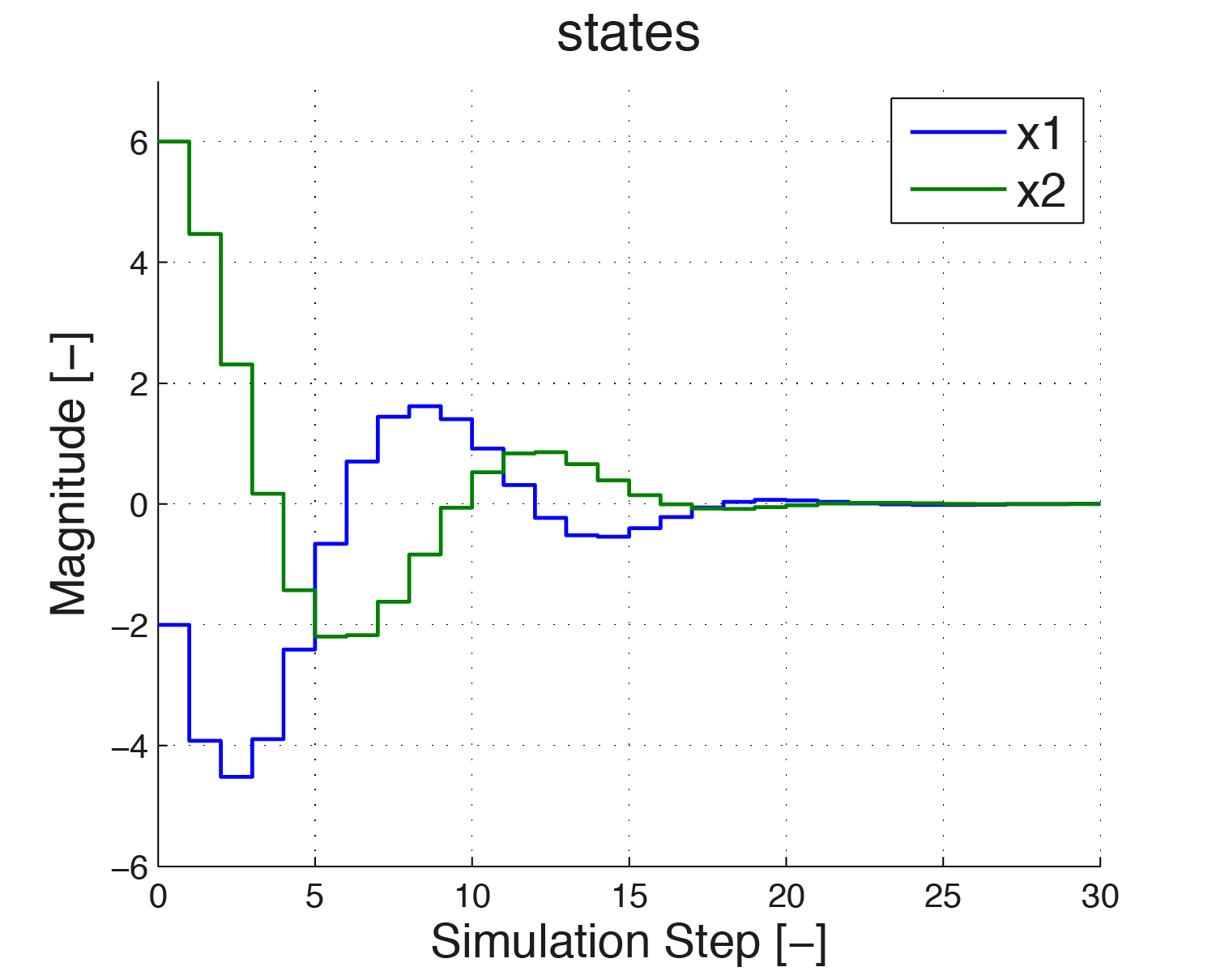
Figure 11.5 The states are both regulated to zero. No constraints are imposed on the states.

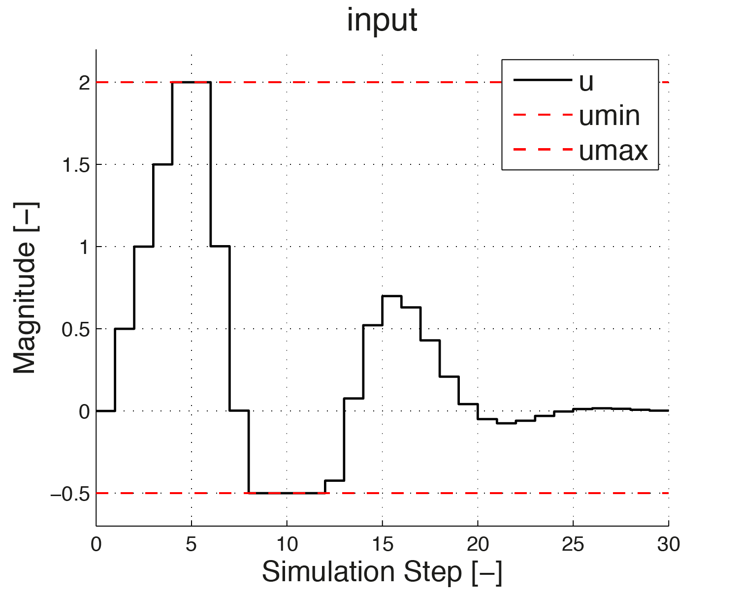
Figure 11.6 Plot of \(u\)

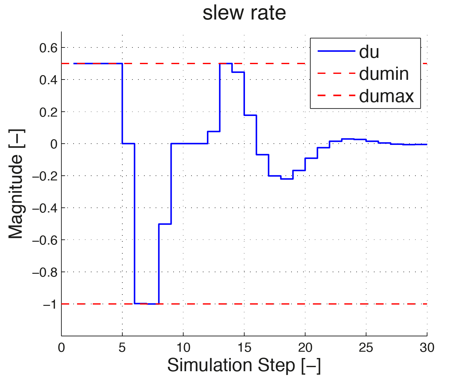
Figure 11.7 Plot of \(du\)

In Figure 11.6 and Figure 11.7 one sees how the input signal is maximally increased in the beginning with a slew rate of \(0.5\), until it reaches its upper bound of 2. In the figure on the right the slew rate is depicted. One can see that in the beginning, the slew rate stays at its upper bound 0.5. At simulation step 6 the input signal is maximally reduced. Again this is visible from the slew rate being at its lower bound \(-1\).