11.1.3. HOW TO: Implement an MPC Controller with a Time-Varying Dynamics
11.1.3.1. Introduction
This ‘HOW TO’ explains how FORCESPRO can be used to handle time-varying models to achieve better control performance than a standard MPC controller. For this example it is assumed that the time-varying model consists of four different systems. This could be four models derived from a nonlinear system at four operating points or from a periodic system. The systems are listed below. The first system is a damped harmonic oscillator, while the second system has eigenvalues on the right plane and is therefore unstable. System three is also a damped oscillator, but differs from system one. System four is an undamped harmonic oscillator.
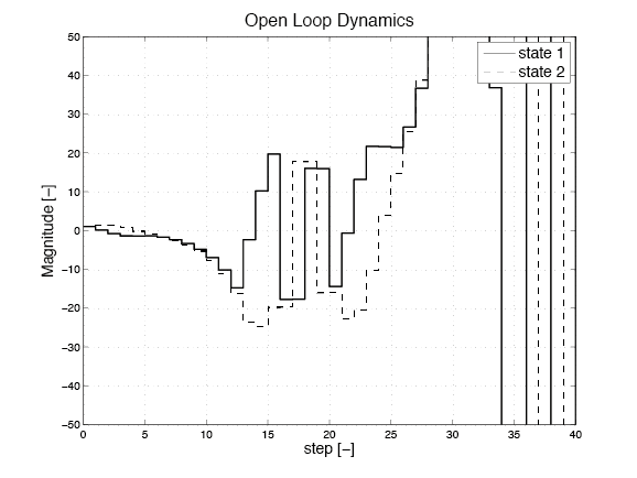
In this example we assume that system 1 is active for the first 4 steps. Then at step 5 the model changes to system 2, which stays active for 8 steps. Then we switch to system 3 for the following 3 steps and finally system 4 is active for the next 5 steps. This pattern is periodic, i. e. every 20 steps the cycle starts again. Also we have an initial condition of \(x_0=[1;1]\), a prediction horizon \(N=15\) and the simulation runs for 40 steps.
The open loop dynamics of this time-varying model are shown on the right. One can see that the system becomes unstable. The goal is to regulate both states to zero while satisfying the different input constraints on each system. The constraints on the model are \(u \in [−3,5]\), \(u \in [−5.5,5.5]\), \(u \in [−3,5]\) and \(u \in [−0.45,4.5]\) for systems 1, 2, 3 and 4, respectively.
At each step \(k\) FORCESPRO takes the changing state space matrices and the corresponding input constraints into account, in order to regulate both states to zero as fast as possible. The following section shows how a controller for this problem can be implemented using the FORCESPRO MATLAB® Interface.
11.1.3.2. Implementation
The FORCESPRO MATLAB® Interface is used to pose a multistage problem problem as described here. When taking the changing dynamics over the prediction horizon into account, the matrices \(C_{i−1}\) and \(D_i\) of the inter-stage equality have to be defined as parameters for each prediction step \(i\). Additionally the lower bounds \(\underline{z}_i\) and the upper bounds \(\overline{z}_i\) on the optimization variable have to be defined as parameters as they also change over the prediction horizon. Also, the initial condition has to be set as a parameter. The code below shows the multistage problem and the commands to design the controller using FORCESPRO.
%% Multistage Problem: Varying Model in Prediction Horizon
stages = MultistageProblem(N); % get stages struct of length N

% Initial Equality
% c_1 = -A*x0
parameter(1) = newParam('minusA_times_x0',1,'eq.c');

for i = 1:N
        % dimension
        stages(i).dims.n = nx+nu; % number of stage variables
        stages(i).dims.r = nx; % number of equality constraints
        stages(i).dims.l = nu; % number of lower bounds
        stages(i).dims.u = nu; % number of upper bounds

        % lower bounds
        stages(i).ineq.b.lbidx = 1; % lower bound acts on these indices
        parameter(1+i) = newParam(['u',num2str(i),'min'],i,'ineq.b.lb');

        % upper bounds
        stages(i).ineq.b.ubidx = 1; % upper bound acts on these indices
        parameter(1+N+i) = newParam(['u',num2str(i),'max'],i,'ineq.b.ub');

        % cost
        stages(i).cost.H = blkdiag(R,Q);
        stages(i).cost.f = zeros(nx+nu,1);

        % Equality constraints
        if( i>1 )
                stages(i).eq.c = zeros(nx,1);
        end
        % Inter-Stage Equality
        % D_i*z_i = [B_i -I]*z_i
        parameter(1+2*N+i) = newParam(['D_',num2str(i)],i,'eq.D');
        if( i < n)
                % C_{i-1}*z_{i-1} = [0 A_i]*z_{i-1}
                parameter(1+3*N+i) = newParam(['C_',num2str(i)],i,'eq.C’);
        end
end

% define outputs of the solver
outputs(1) = newOutput('u0',1,1);
% solver settings
codeoptions = getOptions('Time_Varying_Model_wP');
% generate code
generateCode(stages,parameter,codeoptions,outputs);
You can download the MATLAB code of this example to try it out for yourself by
clicking here.
11.1.3.3. Comparison of the two approaches
The two plots in Figure 11.3 and Figure 11.4 respectively, show the difference between the response of a controller that assumes constant matrices \(A\) and \(B\) over the whole prediction horizon, and a controller that considers the changing dynamics, e. g. at time step 0 the second controller knows that system 1 will only be active for the first 4 steps. The left plot shows the system response and the right plot shows the actuator signals and the varying system constraints.
Both controllers can satisfy the constraints. To quantify the improvement in control performance, the cost function \(\sum_{k=1}^N x_k^T Q x_k + u_k^T R u_k\) can be evaluated for the whole simulation length of \(n=40\). For the controller that uses a fixed model for the prediction horizon, the closed loop cost for regulating the states to zero is 2163.2. With the FORCESPRO time-varying controller the costs is reduced to 457.5. This is a cost reduction of almost 80%.
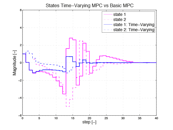
Figure 11.3 States Time-varying MPC vs. basic MPC
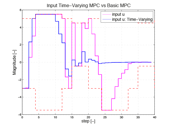
Figure 11.4 Input Time-varying MPC vs. basic MPC