11.1.2. How to Incorporate Preview Information in the MPC Problem
11.1.2.1. Introduction
In this example the following discrete-time system is considered:
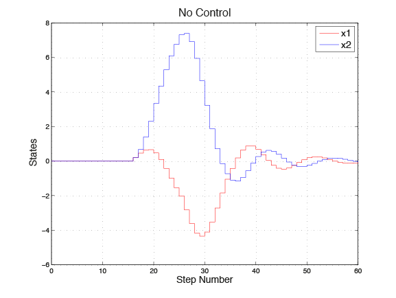
The control objective is to regulate the two states to zero using the input \(u_k\), while a disturbance \(w_k\) is acting on the system. The disturbance \(w_k\) gets predicted for a horizon of length \(N=10\), which is equal to the control horizon of the model predictive control problem solved at each time step by the FORCESPRO controller. At each time step \(k\), a predicted disturbance for the next \(N\) steps is considered by the FORCESPRO controller. For the cost function of the MPC problem, it is assumed that the relative importance of regulating the two states to zero is ten times as high as the penalty on applying an input. Further it is demanded, that the input magnitude of the input signal \(u\) lies in the range \([−1.8,1.8]\). The initial state of the system is set to zero, i. e. \(x_0=[0;0]\).
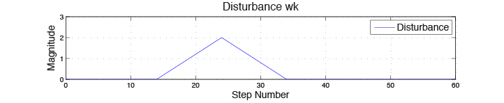
One can see that the disturbance drives the states far away from the desired value. In this example it is shown how FORCESPRO can significantly improve the dynamical behavior by using the concept of ‘preview’ when such future information is available.
11.1.2.2. Use preview information in the MATLAB® interface
The multistage problem is constructed as shown in the simple example here and is then extended as shown below.
The parametric additive terms g have to be defined. At each stage of the multistage problem, the
equality constraint change, therefore we have to define a parameter for each stage. In the definition of the parameters, distx
represents the name of the predicted disturbance at stage x of the multistage problem.
During runtime, the preview information is mapped to these parameters.
% RHS of first eq. constr. is a parameter: z1=-A*x0 -Bw*Road
parameter(1) = newParam('minusA_times_x0_BwDist',1,'eq.c');
% Parameter of Preview
parameter(2) = newParam('dist1',2,'eq.c');
parameter(3) = newParam('dist2',3,'eq.c');
parameter(4) = newParam('dist3',4,'eq.c');
parameter(5) = newParam('dist4',5,'eq.c');
parameter(6) = newParam('dist5',6,'eq.c');
parameter(7) = newParam('dist6',7,'eq.c');
parameter(8) = newParam('dist7',8,'eq.c');
parameter(9) = newParam('dist8',9,'eq.c');
parameter(10) = newParam('dist9',10,'eq.c');
After setting up the multistage problem with the parametric equality constraints, configure the solver settings (i. e. define solver
output and solver options), the solver can be generated by using the command generateCode(...). With the function provided by
FORCESPRO, the system is now ready for simulation.
You can download the MATLAB code of this example to try it out for yourself by
clicking here.
11.1.2.3. Comparison of MPC with Preview and Standard MPC
Figure 11.2 shows the dynamics of the system using a non-preview controller and a preview controller designed using FORCES Pro. One can see that the maximum deviation of the two states from their desired value is reduced by a factor 18, and 11, respectively. Compared to the open loop case, the magnitude of the deviation is reduced by a factor of 47, and 34, respectively.
Figure 11.1 shows the control action of both controllers. As expected, the input signal remains in the allowed range. One can see how the preview controller makes use of future information to provide a more aggressive control action that results in improved system performance.
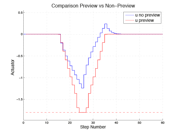
Figure 11.1 Comparison preview vs. non-preview
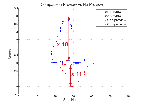
Figure 11.2 Comparison preview vs. no preview