11.7. Low-level interface: DC/DC converter

11.7.1. Example Overview

The example starts by describing the power electronics of the DC/DC converter and how the control oriented model of the system is derived. Then the potential advantages of model predictive control over a conventional PI controller are discussed. Afterwards the design of the MPC controller using FORCESPRO is presented. Finally, the simulation setup is explained and the simulation results using PI and MPC are compared.

• Introduction: General introduction to the example.

• Control Objective: What can be gained by applying MPC with FORCESPRO.

• MPC via FORCESPRO: How to generate a solver with FORCESPRO for the power electronic converter.

• Simulation: Illustration on how to simulate the system with the generated controller.

• Comparison: Discussion of the results of the simulation.

11.7.2. Special Requirements

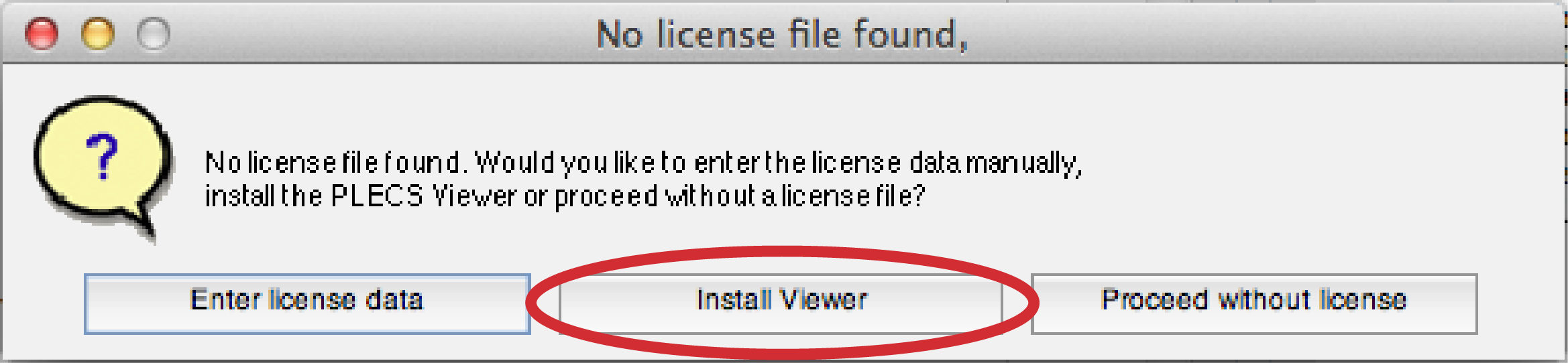
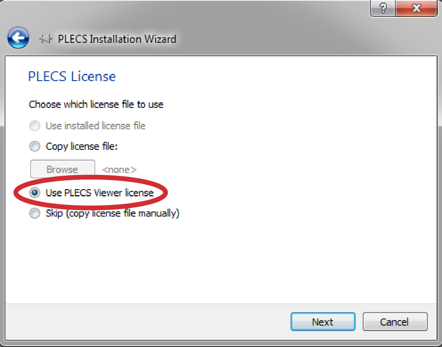
For the simulation of the power electronic converter in this example PLEXIM provided their software PLECS®. PLECS® is the tool for high-speed simulations of power electronic systems. To simulate this example, PLECS Blockset with a viewer license is required. Please follow the instructions on how to install PLECS® below.

PLECS Blockset installation instructions:

• Download PLECS® Blockset installation script available from here.

• Download the required PLECS® Blockset package file here and save it in the same directory as the file installplecs.m.

• Run the file installplecs.m in MATLAB® from the command line.

• During the installation a dialog asks where to save ‘PLECS’. Choose a location which is in the MATLAB® search path.

• During the installation a dialog asks for a license. Install the ‘viewer license’ as shown in the figures below.

Once the installation is completed you are ready to simulate the files provided with this example.

11.7.3. Introduction - Control of a DC/DC Converter

An important field of application for model predictive control are power electronic systems. In this example a typical DC/DC converter which supplies an isolated DC voltage to a telecom system is considered. Assume that the input voltage of the two-transistor forward converter, depicted below on the left, is a constant voltage \(U_{IN}\) delivered by a previous PFC rectifier stage. The load attached to the converter has an ohmic-capacitive characteristic.

This two-transistor forward converter can be modelled as a buck converter from which it is more convenient to derive a control oriented model. The buck converter has only one switch and the input voltage \(U_{in}\) is the actual input voltage scaled by the transformer turn ratio. The equivalent circuit is depicted on the right in the figure below.

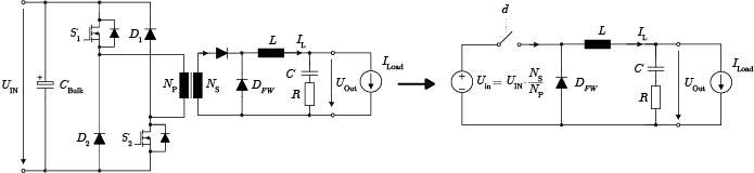
Figure 11.27 Based on the lecture material Power Electronic Systems II, Institute for Power Electronic Systems, ETH Zürich

The states of the control oriented model, which is used as a model for the predictive controller, are the inductor current \(i_L\) and the capacitor voltage \(u_C\). Further there are the input signal d and the disturbances in the input voltage and the load current \(w = \begin{pmatrix} u_{in} & i_{Load} \end{pmatrix}^T\). As an output signal the states \(i_L\) and \(u_C\) as well as the output voltage uout are considered. The small signal model (small signals are marked with a hat) in state-space form reads as:

\begin{align*} \frac{d}{dt}\hat{x} & = \begin{pmatrix} -\tfrac{R}{L} & -\tfrac{1}{L} \\ \tfrac{1}{C} & 0 \end{pmatrix}\hat{x} + \begin{pmatrix} \tfrac{U_{in}}{L} \\ 0 \end{pmatrix}\hat{d} + \begin{pmatrix} \tfrac{D}{L} & -\tfrac{R}{L} \\ 0 & -\tfrac{1}{C} \end{pmatrix}\hat{w} \\ \hat{y} & = \begin{pmatrix} 1 & 0 \\ 0 & 1 \\ R & 1 \end{pmatrix}\hat{x} + \begin{pmatrix} 0 & 0 \\ 0 & 0 \\ 0 & -R \end{pmatrix}\hat{w} \\ \\ & \quad \quad \quad \quad \Big\Updownarrow \\ \\ \frac{d}{dt}\hat{x} & = A\cdot \hat{x} + B1\cdot u + B2\cdot \hat{w} \\ \hat{y} & = C \cdot \hat{x} + \begin{pmatrix} D2 \\ D4 \\ \end{pmatrix} \cdot \hat{w} \end{align*}

11.7.4. Control Objective by Using Model Predictive Control

The converter should provide a constant output voltage \(U_{Out}\) of 60 V while delivering the power required by the load. The nominal load current \(I_{Load}\) is 22 A. The input voltage \(U_{in}\) is constant at level 144 V, while the load resistance varies in the range \([1.5, 5] \Omega\).

Conventionally the output voltage of the Buck Converter was controlled by a PI controller. In the first plot below, the current \(i_L\) in the inductor is shown, when the resistance in the load is reduced from \(5 \Omega\) to \(1.5 \Omega\), i. e. from upper bound to the lower bound of the possibly required load resistance. The red curve represents the current in the inductor. Also the change in the output voltage is depicted when changing the load resistance.

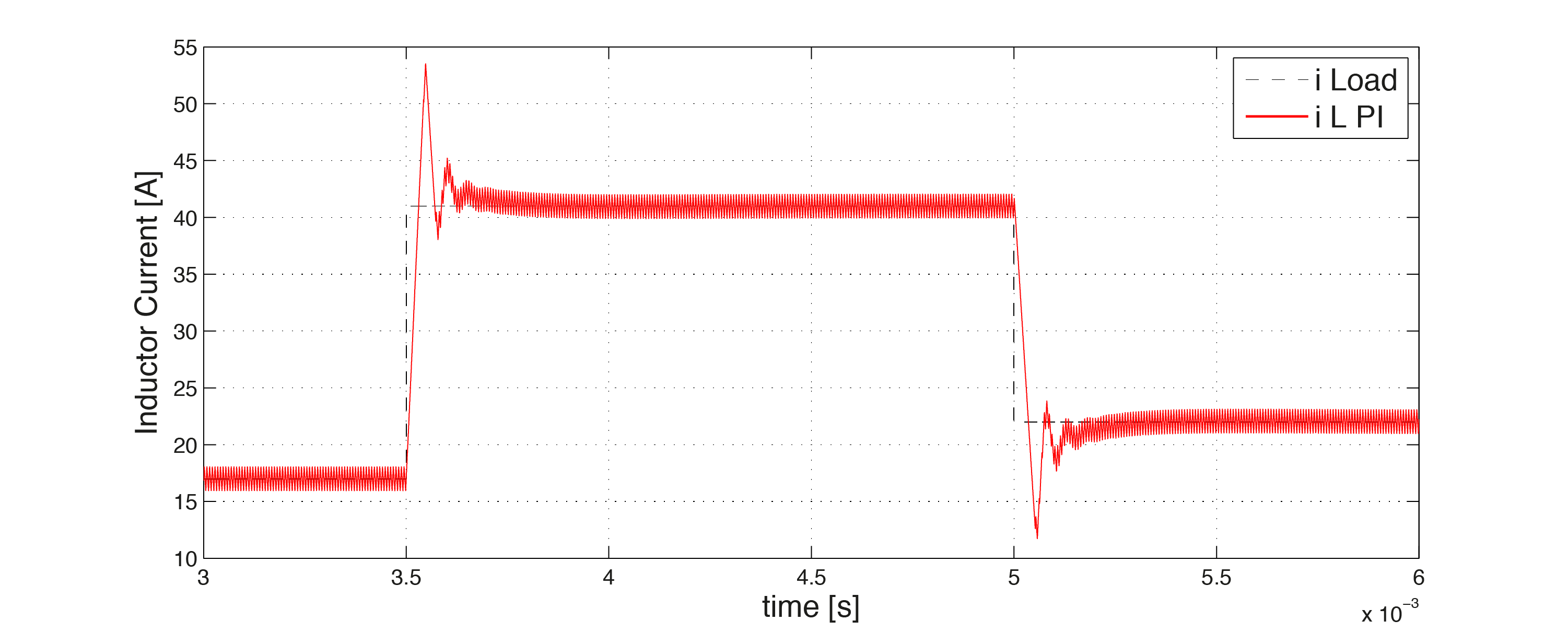
Figure 11.28 Inductor current vs. time

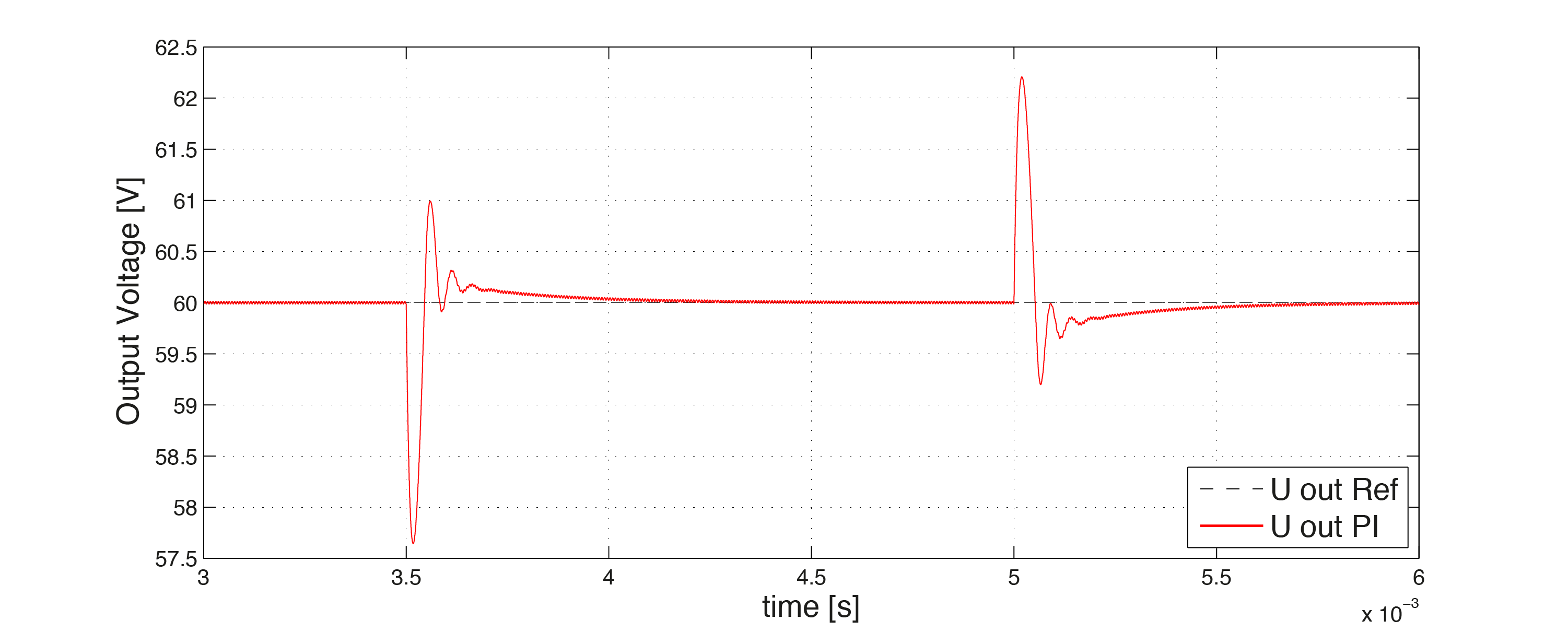
Figure 11.29 Output voltage vs. time

From Figure 11.28 and Figure 11.29 one can see that the current in the inductor has a high overshoot and the output voltage has a relatively long settling time when a change in the load resistance occurs.

Important

Some of the potential benefits of model predictive control are the following

• Below it is shown that the size of the converter can be reduced by using a MPC controller designed with FORCESPRO. With the MPC controller it will be possible to limit the current in the inductor. With the warranty that the current does not exceed a certain upper bound, a smaller inductor can be built in and the costs are reduced.

• Also the controller designed with FORCESPRO will calculate the optimal input at every time step. The performance of the system is increased, i. e. less overshoot and faster settling time.

11.7.5. Model Predictive Control Design via FORCESPRO MATLAB® Interface

To design the FORCESPRO controller, the MPC setup has to be defined first. Below the requirements are shown. A prediction horizon of 25 is chosen. In the cost function \(R\) penalizes the deviation of the input signal from its reference value. The matrix \(Q\) penalizes the deviation of the states from its reference values. Notice that \(Q\) is defined such that a deviation of the inductor current to its reference value is less penalized than a deviation of the output voltage to its reference value. The input signal \(d\) to the PWM is limited to [0, 1], while the inductor current should not exceed a current of 42 A. This overshoot limitation concerns the average inductor current. Below one can see, that this limit is exceeded by half of the currents peak-to-peak value. The constraints are consistently defined with the model, i. e. a current reduction by -20 A and a current enhancement by 20 A is allowed at most. This is equivalent to a current in the inductor in the range of [2, 42] A.

% MPC Setup
N = 25;
Q = [.01, 0; 0, 10];
R = 1;
nx = 2;
nu = 1;

% Constraints
umin = 0;
umax = 1;
xmin = -20;
xmax = 20;

Next, the multistage problem is formulated. In this example, there exists a linear term \(f\) in the cost function due to the variable load, i. e. the steady-state inductor current changes. The cost function therefore reads as

\[(x^{+} - x_{ref})^{T} Q (x^{+} - x_{ref})+(u - u_{ref})^{T} R(u - u_{ref})\]

To solve the optimization problem, the reference values need to be re-calculated at every time step. Below the parameters of the problem are marked red. The optimization variable of the multistage problem is \(z_i = \begin{pmatrix} u_i & x_{i+1} \end{pmatrix}^T\), where \(u\) is the input signal given to the system.

\begin{align*} \text{minimize}& \quad \sum_{i=1}^N \frac{1}{2}z_i^T H_i z_i + f_i^T z_i &\text{(separable objective)} \\ \text{subject to}& \quad D_1 z_1 = c_1 &\text{(initial equality)} \\ & \quad C_{i-1}z_{i-1}+D_iz_i = c_i & \text{(inter-stage equality)} \\ & \quad \underline{z}_i \leq z_i \leq \overline{z}_i & \text{(bounds)} \end{align*}

In this example three parameters have to be given to the solver.

• parameter(1): Represents the right hand side of the initial equality of the problem in standard form above.

• parameter(2): The linear term \(f\) of the cost function. This term contains the reference values of the states which are calculated based on the resistance of the load.

• parameter(3): Represents the right hand side of the inter-stage equality constraint for the stages \(i = 2:N\) of the problem.

Next to the parameters, the dimensions of the variables, the equality constraints and the bounds have to be defined. The values defined in the MPC setup are added to the multistage problem in the section ‘cost’. The terms in the equality constraints which are constant over all stages are defined in the section ‘equality constraints’. After defining the output of the solver and the solver settings, the code for the controller can be generated.

%% Multistage Problem
% get stages struct of length N
stages = MultistageProblem(N);

% RHS of first eq. constr. is a parameter: stages(1).eq.c = -A*x0 - B2*w
parameter(1) = newParam('minusAx0_minusB2w',1,'eq.c');

% Linear Term depends on x_ref and u_ref
parameter(2) = newParam('Linear_Term',1:N,'cost.f');

% RHS of equality constraints for remaining stages: stages(i).eq.c = - B2*w
parameter(3) = newParam('minusB2w',2:N,'eq.c');


for i = 1:N

   % dimension
   stages(i).dims.n = nx+nu;  % number of stage variables
   stages(i).dims.r = nx; % number of equality constraints
   stages(i).dims.l = 2; % number of lower bounds
   stages(i).dims.u = 2; % number of upper bounds

   % cost
   stages(i).cost.H = blkdiag(R,Q);

   % lower bounds
   stages(i).ineq.b.lbidx = 1:2; % lower bound acts on these indices
   stages(i).ineq.b.lb = [umin; xmin]; % lower bound on input u and state iL

   % upper bounds
   stages(i).ineq.b.ubidx = 1:2; % upper bound acts on these indices
   stages(i).ineq.b.ub = [umax; xmax]; % upper bound on input u and state iL

   % equality constraints
   if( i < N )
          stages(i).eq.C = [zeros(nx,nu), Ad];
   end
   stages(i).eq.D = [Bd1, -eye(nx)];
end

% define outputs of the solver
outputs(1) = newOutput('u0',1,1);

% solver settings
codeoptions = getOptions('DCDC_FORCES_Pro_Controller');

% generate code
generateCode(stages,parameter,codeoptions,outputs);

You can download the MATLAB code of this example to try it out for yourself by clicking here.

11.7.6. Simulation of the PLECS® Model with Model Predictive Control

After the code is generated, the FORCESPRO Simulink® block can be added to the model DCDC_FORCES_Pro_viewer.slx as shown in the figure below (copy/paste it from the file DCDC_FORCES_Pro_Controllercompact_lib.mdl in the folder DCDC_FORCES_Pro_Controller/Interface generated by FORCESPRO).

The controller has a frequency of 100 kHz. To simulate the system with a time step of \(1e-7 s\), rate transition blocks are used. Below the Simulink® model DC_DC_FORCES_Pro.slx with the PLECS® circuit and the FORCESPRO controller is depicted.

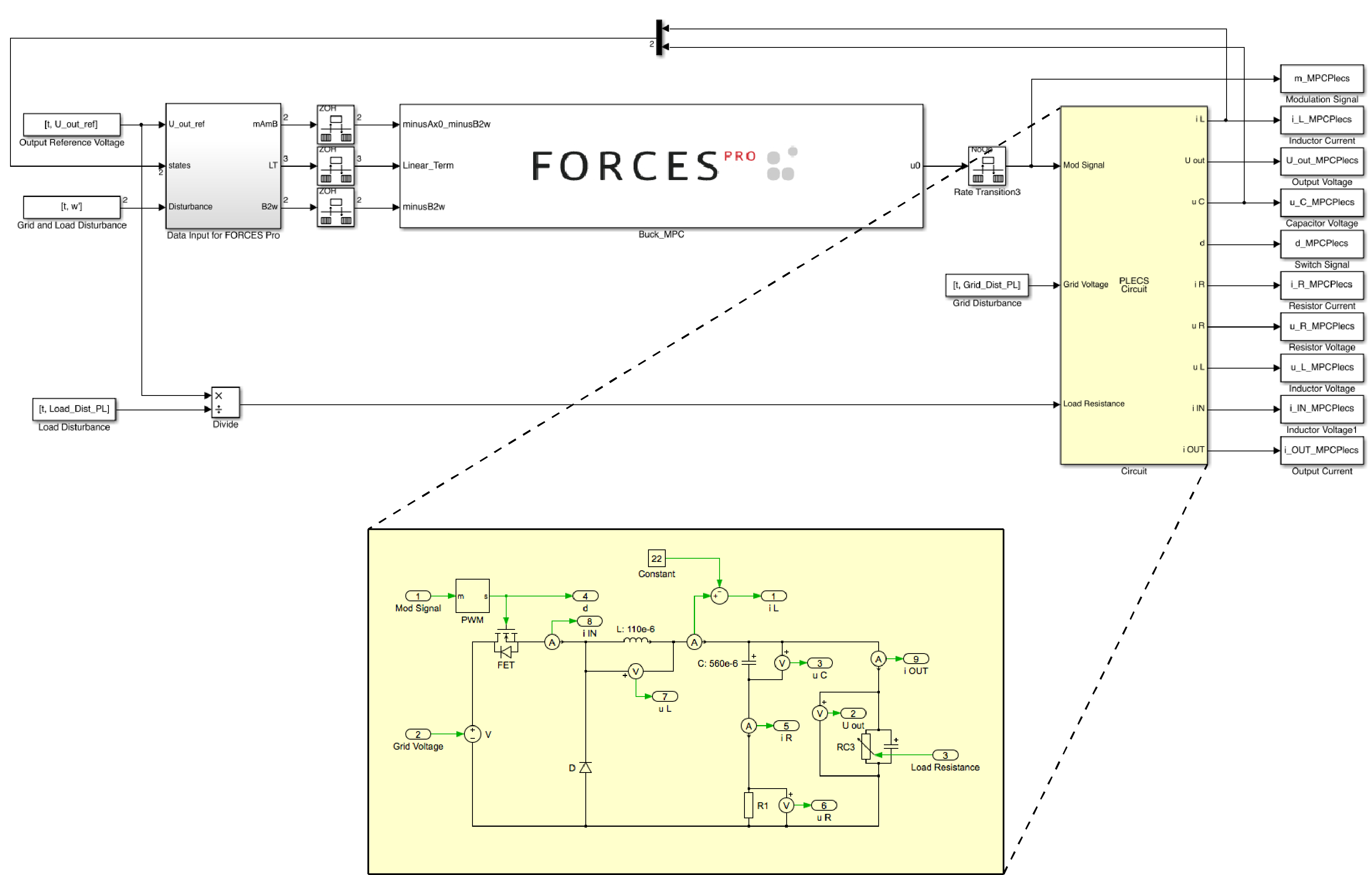
In the grey box in the model depicted above, the three parameters which are the input to the FORCESPRO controller, are calculated.

• parameter(1): The right hand side of the initial equality constraint is \(-Ad \cdot x -Bd2 \cdot w\).

• parameter(2): For the linear term of the cost function the reference values for the states and the input signal need to be calculated.

The reference values are calculated by solving the linear system

\[\begin{split}\begin{pmatrix} Ad−I & Bd1 \\ Cd2 & Dd3 \end{pmatrix} \cdot \begin{pmatrix} x_{ref} \\ u_{ref} \end{pmatrix}= \begin{pmatrix} −Bd2\cdot w \\ U_{out,ref}−Dd4\cdot w \end{pmatrix}\end{split}\]

which follows from the system equations in steady-state. To calculate the linear term f the reference values are plugged into the linear term \(f= \begin{pmatrix} −u_{ref} \cdot R & −x_{ref}^T \cdot Q \end{pmatrix}^T\), which is equal to

\begin{equation*} f = \begin{pmatrix} Ad−I & Bd1 \\ Cd2 & Dd3 \end{pmatrix}^{-1} \cdot \begin{pmatrix} 0 & -Bd2 \\ 1 & -Dd4 \end{pmatrix} \cdot \begin{pmatrix} U_{out, ref} \\ w \end{pmatrix} \cdot \begin{pmatrix} 0 & -R \\ -Q & 0 \end{pmatrix} \end{equation*}

The matrices in the derivation above are explained in more detail in the system presented in the code available for this example.

• parameter(3) is equal to \(-Bd2 \cdot w\).

11.7.7. Comparison of Model Predictive Control and PI Control

In the Figure 11.30 and Figure 11.31 below the evolution of the inductor current and the output voltage are compared when controlling the system with PI and with the MPC controller designed using FORCESPRO. It can be seen that the MPC controller is able to keep the inductor current within the limits defined above. However, this limits the tracking speed of the output voltage in the corresponding time interval. Overall, the tracking performance of the output voltage is increased compared to the baseline PI controller.

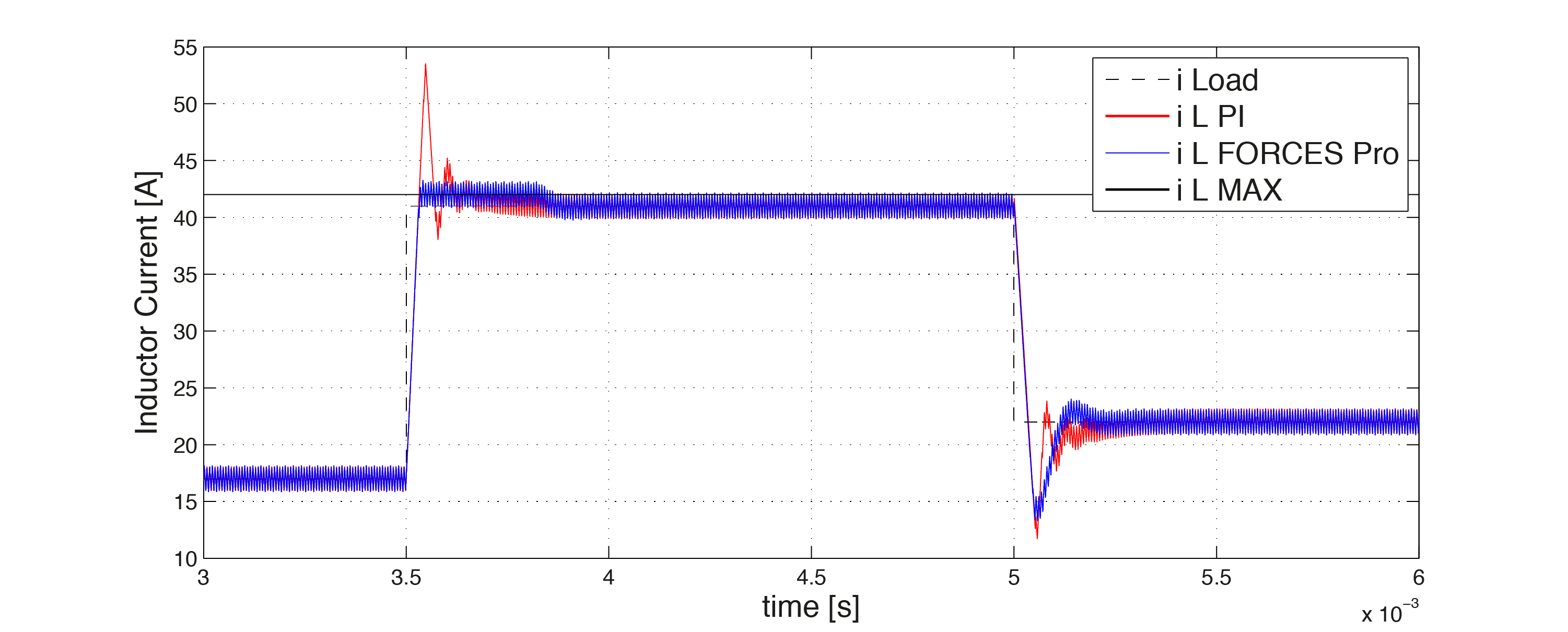
Figure 11.30 Inductor current vs. time

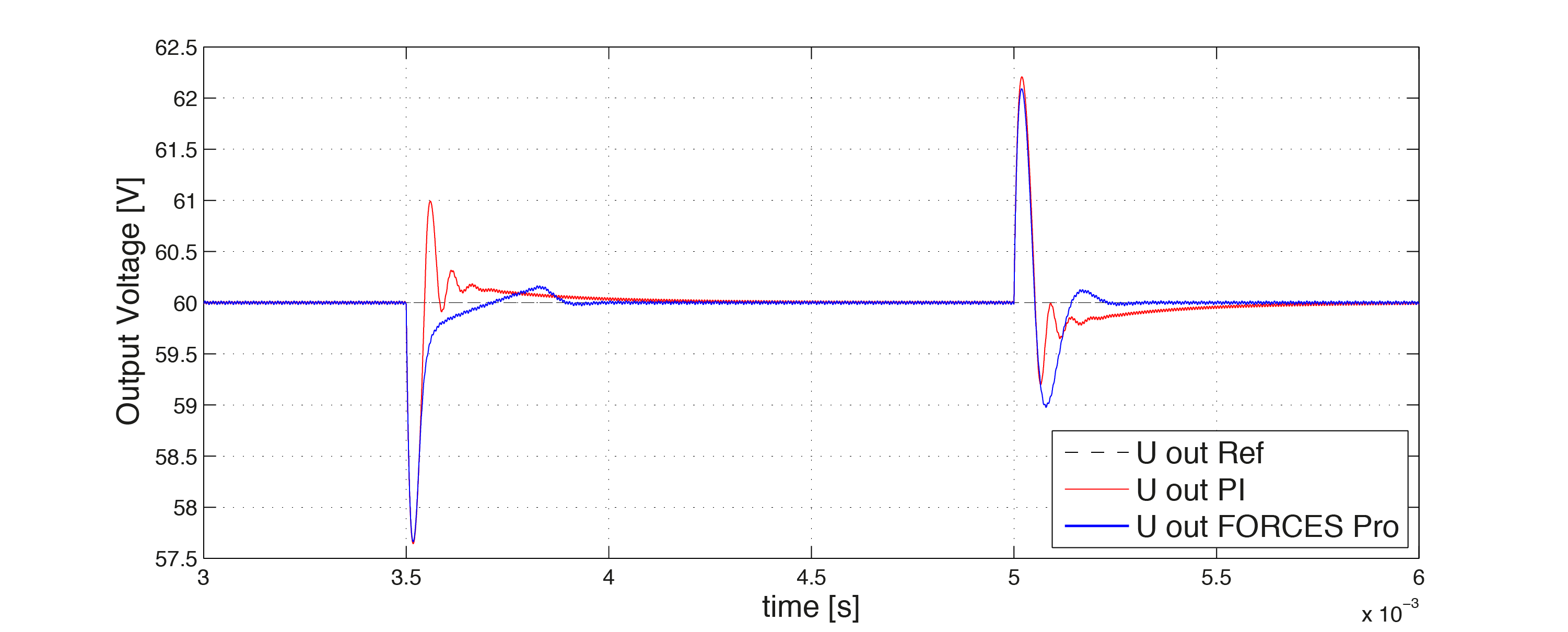
Figure 11.31 Output voltage vs. time