11.5. Low-level interface: Robust estimation (Kalman filter)
11.5.1. System Description
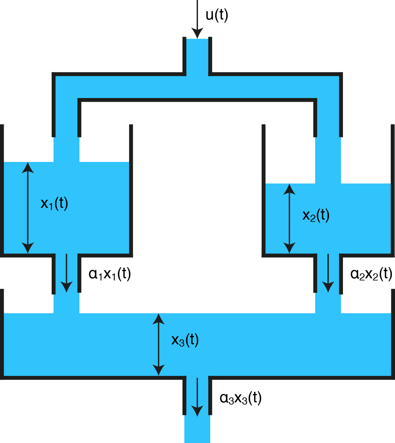
In this example we consider the water tank system depicted on the right. Tank 1 has one input flow and one output flow. Also tank 2 has one input flow and one output flow. Tank 3 has two input flows and one output flow. The system dynamics are represented via the first equation below. As an output \(z\) we have a measurement of the level of tank 1 and of the level of tank 3.
The states of the system are \(x= \begin{pmatrix} x_1 & x_2 & x_3 \end{pmatrix}^T ` and as an input the flow :math:`u\) is given. There is a process noise \(v\) and a measurement noise \(w\), both are Gaussian Random Variables with mean \(0\) and variance \(Q\) and \(R\), i. e. \(v \sim \mathcal{N}(0,Q)\) and \(w \sim \mathcal{N}(0,R)\). The sparse signal \(y\), which is used to model sensor failures, distorts the measurement signal additionally.
The goal of this example is to show, that the standard Kalman Filter is not working that good anymore if sensor failures are present. There does not exist an analytic solution to the problem if the disturbance \(y\) is present. Using the robust Kalman Filter, i. e. replacing the standard measurement update step with an extended optimization problem, which is solved by FORCESPRO, the filter is robust against \(y\) and the estimated states are much more accurate compared to the standard Kalman Filter. To process the measurement data online, the optimization problem has to be solved in a sufficiently short amount of time.
11.5.2. Robust Kalman filter
Recall that the standard Kalman Filter, which would be applied if disturbance signal \(y\) were not present, consists of two steps: First a prediction step is made, where a predicted stated \(x^p(k)\) is calculated based on the estimated state \(x^m(k-1)\). Additionally, the predicted variance \(P_p(k)\) gets calculated in the prediction step. The measurement step returns the variance \(P_m(k)\) and the state estimate \(x^m(k)\). This state estimate \(x^m(k)\) is basically the solution of the optimization problem
In this example, we assume that out of 100 measurements the sensors of tank 1 gand tank 3 gives each 5 bogus signals. In order to make the state estimator robust against the sensor failures \(y\), we solve the following convex optimization problem at every time instance
In the optimization problem \(w\), \(x\) and \(y\) are optimization variables. The cost function of the optimization problem is extended with the \(l_1\)-penalty which is non-quadratic. The value \(\lambda \geq 0\) is a tuning parameter. For \(\lambda\) large enough, the solution of the optimization problem has \(y=0\) and therefore the estimates of the robust Kalman Filter coincides with the standard Kalman Filter solution. This optimization problem can be transformed as described in here. We transform this problem to the form required by FORCESPRO, which reads as
where the optimization variable is given by \(\tilde{z}=\begin{pmatrix} x^T & w^T & y^T & e^T \end{pmatrix}^T\). Please find below the MATLAB code to generate the solver for the optimization problem with FORCESPRO. The covariance matrix \(P^{-1}\) is updated at every time step and therefore the problem can’t be solved explicitly. In this problem three parameters need to be defined, which are \(H\), \(f\) - containing the predicted covariance and the predicated state - and \(c\) - contains the current measurement.
%% Create FORCESPRO Solver for Measurement Update Step
% assume variable ordering z = [x,w,y,e]

% Create multistage struct
stages = MultistageProblem(1);

% Dimension
[ny nx] = size(H);
nw = ny;
ne = ny;
stages(1).dims.n = nx+nw+ny+ne; % number of stage variables
stages(1).dims.r = ny;          % number of equality constraints
stages(1).dims.p = 2*ne;        % number of polytopic constraints

% Polytopic bounds
stages(1).ineq.p.A = [zeros(ny,nx), zeros(ny,nw), lambda*eye(ny), -eye(ne); ...
                      zeros(ny,nx), zeros(ny,nw), -lambda*eye(ny), -eye(ne)];
stages(1).ineq.p.b = zeros(2*ne,1);

% Equality constraints
stages(1).eq.D = [H, eye(nw), eye(ny), zeros(ne)];

% Parameters
params(1) = newParam('H_i',1,'cost.H');
params(2) = newParam('f_i',1,'cost.f');
params(3) = newParam('z_i',1,'eq.c');

% Output
outputs(1) = newOutput('x_hat_RKF',1,1:3);

% Code Generation
codeoptions = getOptions('Robust_KF');
generateCode(stages,params,codeoptions,outputs);
You can download the MATLAB code of this example to try it out for yourself by
clicking here.
11.5.3. Simulation and Comparison
In the simulation the optimization problem has to be solved at every time instance. In the prediction step the state \(x^p\) is calculated
based on the estimation of the current state. Also the the variance is updated in every prediction step. In the measurement update step the
estimated state \(x^m\) is calculated based on the predicted state, its predicted variance and the current measurement \(z\) by the
function Robust_KF() generated by FORCESPRO.
for i = 2:(N+1)

    % Prediction Step
    x_p_RKF = Ak(:,:,i-1)*x_hat_RKF(:,i-1)+B*u(i-1);
    P_p_RKF(:,:,i) = Ak(:,:,i-1)*P_hat_RKF(:,:,i-1)*Ak(:,:,i-1)' + Q;

    % Measurement Update Step - Optimization Problem
    problem.H_i = [2*inv(P_p_RKF(:,:,i)),zeros(nx,nw+ny+ne); ...
                   zeros(ny,nx),2*R_inv,zeros(ny,ny+ne); ...
                   zeros(ny+ne,nx+nw+ny+ne)];
    problem.f_i = [-2*(inv(P_p_RKF(:,:,i))*x_p_RKF); ...
                   zeros(nw,1); ...
                   zeros(ny,1); ...
                   ones(ne,1)];
    problem.z_i = z(:,i);
    [solverout,~,info] = Robust_KF(problem);
    solve_time(i-1) = info.solvetime;
    P_hat_RKF(:,:,i) = P_p_RKF(:,:,i);
    x_hat_RKF(:,i) = solverout.x_hat_RKF;

end
In the plots in Figure 11.19, Figure 11.20 and Figure 11.21 respectively, the estimated states are depicted. The estimates calculated via the robust Kalman Filter, in blue, are much more accurate then the standard approach. The peaks in the red line indicate sensor failures against which the standard Kalman Filter is not robust.
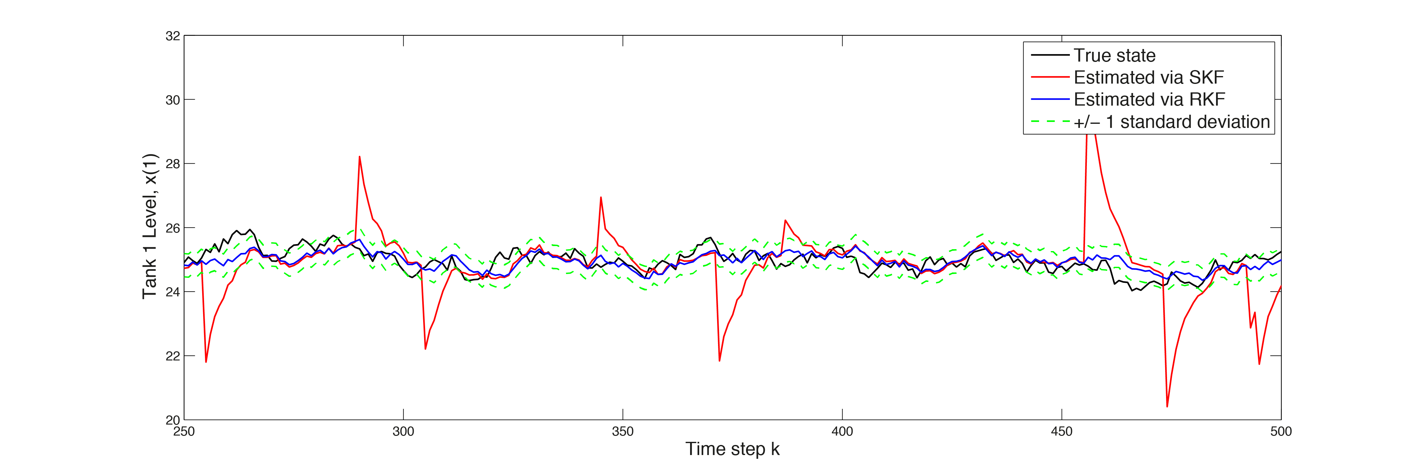
Figure 11.19 Estimated state \(x(1)\)
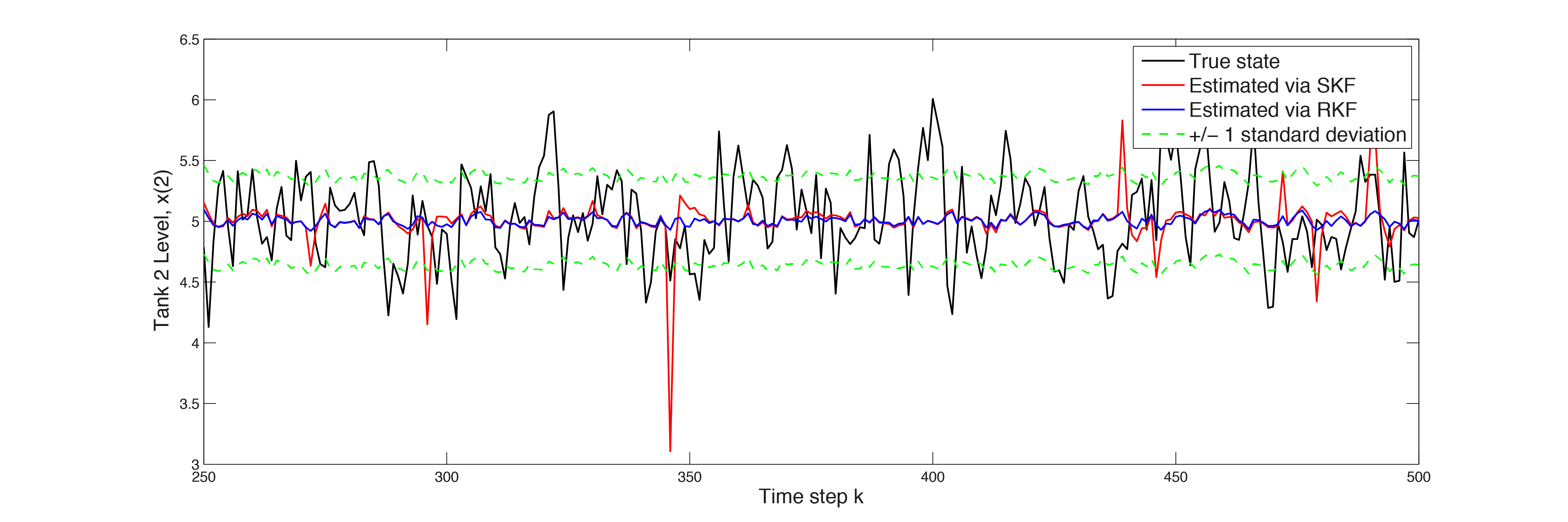
Figure 11.20 Estimated state \(x(2)\)
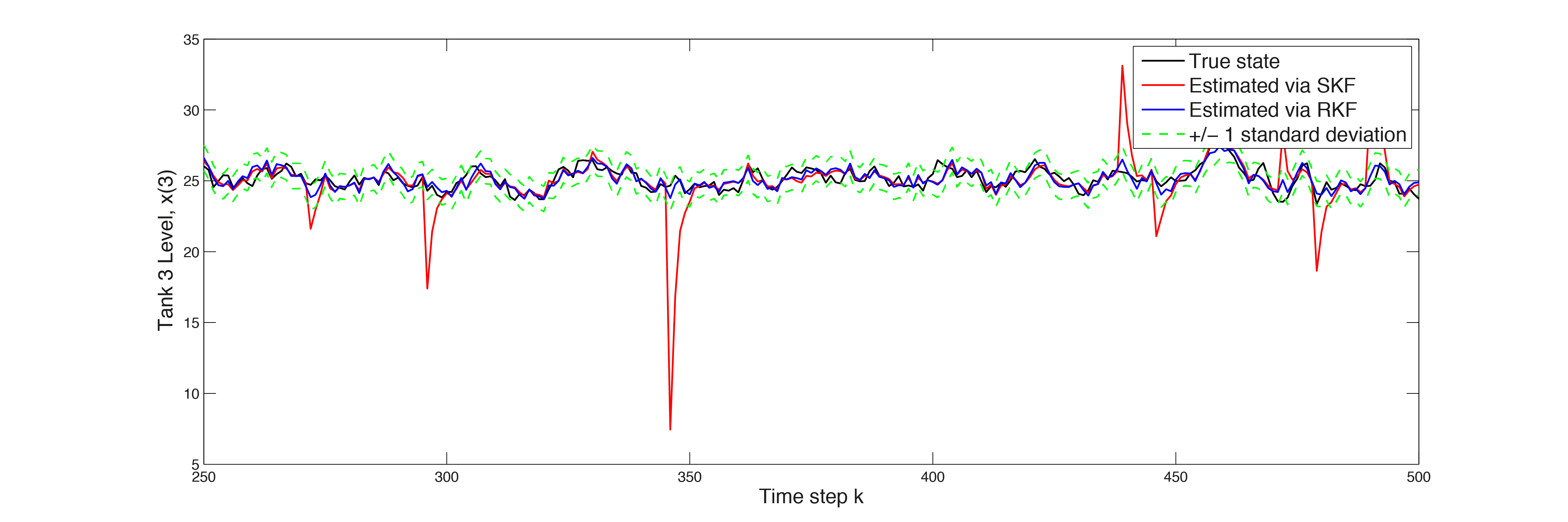
Figure 11.21 Estimated state \(x(3)\)
The impact on the RMS error magnitude of the robust Kalman Filter can be seen in the plots in Figure 11.22, Figure 11.23 and Figure 11.24. The magnitude of the robust Kalman Filter depicted in blue, is reduced by \(\sim 65\%\) for state 1, \(\sim 12\%\) for state 2, \(\sim 61\%\) for state 3 (this values vary). Applying online optimization with FORCESPRO improves the quality of the state estimations significantly.
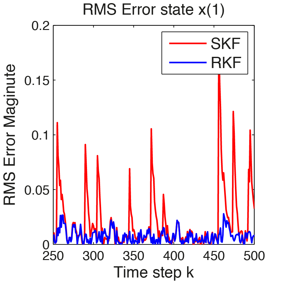
Figure 11.22 RMS error for \(x(1)\)
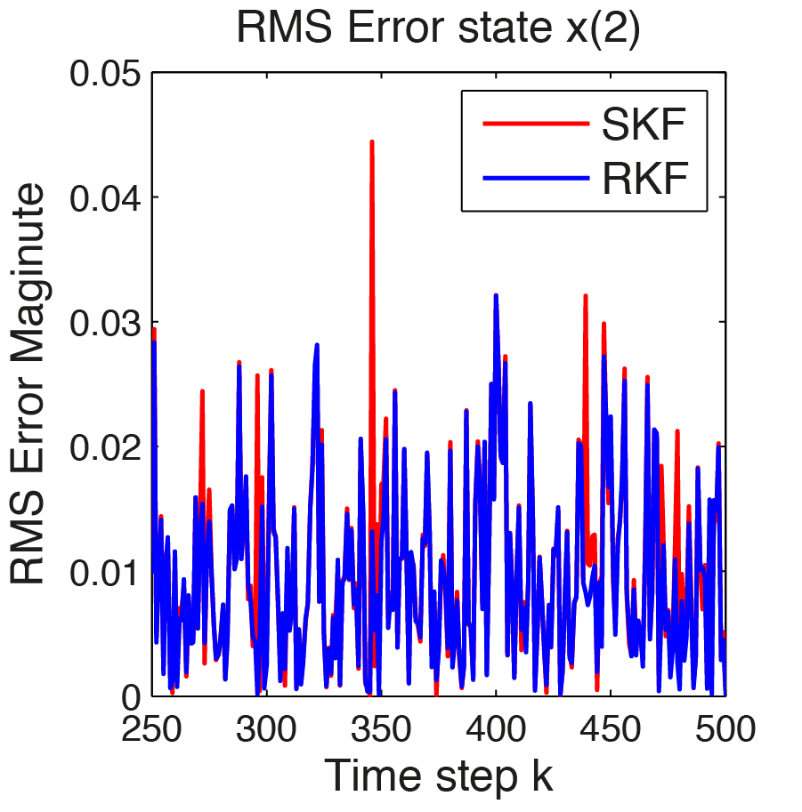
Figure 11.23 RMS error for \(x(2)\)
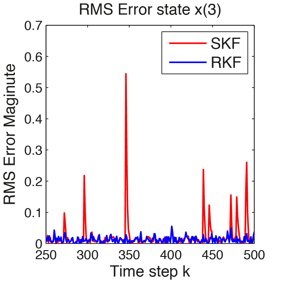
Figure 11.24 RMS error for \(x(3)\)
With FORCESPRO convex optimization can be embedded directly in signal processing algorithms that run online, with strict real-time deadlines, even at rates of tens of kilohertz. In this example the optimization problem is solved in \(\sim 0.1ms\).