11.2. Y2F interface: Basic example
Consider the following linear MPC problem with lower and upper bounds on state and inputs, and a terminal cost term:
This problem is parametric in the initial state \(\color{red} x\) and the first input \(u_0\) is typically applied to the system after a solution has been obtained. Here we present the problem formulation with YALMIP, how you can use Y2F to easily generate a solver with FORCESPRO, and how you can use the resulting controller for simulation.
You can download the MATLAB code of this example to try it out for yourself from https://raw.githubusercontent.com/embotech/Y2F/master/examples/mpc_basic_example.m.
Important
Make sure to have YALMIP installed correctly (run yalmiptest to verify
this).
11.2.1. Defining the problem data
Let’s define the known data of the MPC problem, i.e. the system matrices \(A\) and \(B\), the prediction horizon \(N\), the stage cost matrices \(Q\) and \(R\), the terminal cost matrix \(P\), and the state and input bounds:
%% MPC problem data

% system matrices
A = [1.1 1; 0 1];
B = [1; 0.5];
[nx,nu] = size(B);

% horizon
N = 10;

% cost matrices
Q = eye(2);
R = eye(1);
if exist('dlqr', 'file')
    [~,P] = dlqr(A,B,Q,R);
else
    fprintf('Did not find dlqr (part of the Control Systems Toolbox). Will use 10*Q for the terminal cost matrix.\n');
    P = 10*Q;
end

% constraints
umin = -0.5;     umax = 0.5;
xmin = [-5; -5]; xmax = [5; 5];
11.2.2. Defining the MPC problem
Let’s now dive in right into the problem formulation:
%% Build MPC problem in Yalmip

% Define variables
X = sdpvar(nx,N+1,'full'); % state trajectory: x0,x1,...,xN (columns of X)
U = sdpvar(nu,N,'full'); % input trajectory: u0,...,u_{N-1} (columns of U)

% Initialize objective and constraints of the problem
cost = 0; const = [];

% Assemble MPC formulation
for i = 1:N
    % cost
    if( i < N )
        cost = cost + 0.5*X(:,i+1)'*Q*X(:,i+1) + 0.5*U(:,i)'*R*U(:,i);
    else
        cost = cost + 0.5*X(:,N+1)'*P*X(:,N+1) + 0.5*U(:,N)'*R*U(:,N);
    end

    % model
    const = [const, X(:,i+1) == A*X(:,i) + B*U(:,i)];

    % bounds
    const = [const, umin <= U(:,i) <= umax];
    const = [const, xmin <= X(:,i+1) <= xmax];
end
Thanks to YALMIP, defining the mathematical problem is very much like writing down the mathematical equations in code.
11.2.3. Generating a solver
We have now incrementally built up the cost and const objects, which are both
YALMIP objects. Now comes the magic: use the function optimizerFORCES to
generate a solver for the problem defined by const and cost with the initial
state as a parameter, and the first input move \(u_0\) as an output:
%% Create controller object (generates code)
% for a complete list of codeoptions, see
% https://www.embotech.com/FORCES-Pro/User-Manual/Low-level-Interface/Solver-Options
codeoptions = getOptions('simpleMPC_solver'); % give solver a name
controller = optimizerFORCES(const, cost, codeoptions, X(:,1), U(:,1), {'xinit'}, {'u0'});
That’s it! Y2F automatically figures out the structure of the problem and generates a solver.
11.2.4. Calling the generated solver
We can now use the controller object to call the solver:
% Evaluate controller function for parameters
[output,exitflag,info] = controller{ xinit };
or call the generated MEX code directly:
% This is an equivalent call, if the controller object is deleted from the workspace
[output,exitflag,info] = simpleMPC_solver({ xinit });
Tip
Type help solvername to get more information about how to call the solver.
11.2.5. Simulation
Let’s now simulate the closed loop over the prediction horizon \(N\):
%% Simulate
x1 = [-4; 2];
kmax = 30;
X = zeros(nx,kmax+1); X(:,1) = x1;
U = zeros(nu,kmax);
problem.z1 = zeros(2*nx,1);
for k = 1:kmax

  % Evaluate controller function for parameters
  [U(:,k),exitflag,info] = controller{ X(:,k) };

  % Always check the exitflag in case something went wrong in the solver
  if( exitflag == 1 )
      fprintf('Time step %2d: FORCES took %2d iterations and %5.3f ', k,  info.it, info.solvetime*1000);
      fprintf('milliseconds to solve the problem.\n');
  else
      info
      error('Some problem in solver');
  end

  % State update
  X(:,k+1) = A*X(:,k) + B*U(:,k);
end
11.2.6. Results
The results of the simulation are presented in Figure 11.8. The plot on the top shows the system’s states over time, while the plot on the bottom shows the input commands. We can see that all constraints are respected.
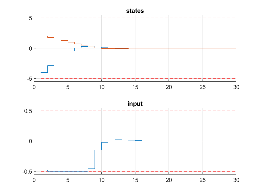
Figure 11.8 Simulation results of the states (top, in blue and red) and input (bottom, in blue) over time. The state and input constraints are plotted in red dashed lines.
11.2.7. Variation 1: Parametric cost
One possible variation is if we consider the weighting matrices \(\color{red} Q\), \(\color{red} R\) and \(\color{red} P\) as parameters, so that we can tune them after the code generation. The following problem is solved at each time step:
As usual, this problem is also parametric in the initial state
\(\color{red} x\) and the first input \(u_0\) is applied to the system
after a solution has been obtained. To be able to define the weighting matrices
\(\color{red} Q\), \(\color{red} R\) and \(\color{red} P\) as
parameters, first we define them as sdpvars and then tell optimizerFORCES
that they are parameters:
% Cost matrices - these will be parameters later
Q = sdpvar(nx);
R = sdpvar(nu);
P = sdpvar(nx);

% [... formulate MPC problem in YALMIP ...]

% Define parameters and outputs
codeoptions = getOptions('parametricCost_solver'); % give solver a name
parameters     = { X(:,1),   Q,   R,   P  };
parameterNames = { 'xinit', 'Q', 'R', 'P' };
outputs     =      U(:,1)   ;
outputNames = {'controlInput'};
controller = optimizerFORCES(const, cost, codeoptions, parameters, outputs, parameterNames, outputNames);
You can download the MATLAB code of this variation to try it out for yourself from https://raw.githubusercontent.com/embotech/Y2F/master/examples/mpc_parametric_cost.m.
11.2.8. Variation 2: Time-varying dynamics
Another possible variation is if we consider the state-space dynamics matrices \(\color{red} A\) and \(\color{red} B\) as parameters, so that we can change them after the code generation. The following problem is solved at each time step:
As usual, this problem is also parametric in the initial state
\(\color{red} x\) and the first input \(u_0\) is applied to the system
after a solution has been obtained. To be able to define the state-space
dynamics matrices \(\color{red} A\) and \(\color{red} B\) as parameters,
first we define them as sdpvars and then tell optimizerFORCES that they
are parameters:
A = sdpvar(nx,nx,'full'); % system matrix - parameter
B = sdpvar(nx,nu,'full'); % input matrix - parameter

% [... formulate MPC problem in YALMIP ...]

% Define parameters and outputs
codeoptions = getOptions('parametricDynamics_solver'); % give solver a name
parameters = { x0, A, B };
parameterNames = { 'xinit', 'Amatrix', 'Bmatrix' };
controller = optimizerFORCES(const, cost, codeoptions, parameters, U(:,1), parameterNames, {'u0'} );
You can download the MATLAB code of this variation to try it out for yourself from https://raw.githubusercontent.com/embotech/Y2F/master/examples/mpc_parametric_dynamics.m.
11.2.9. Variation 3: Time-varying constraints
One final variation is if we consider the constraint inequalities as parameters, so that we can change them after the code generation. The inequalities are defined by a time-varying \(2 \times 2\) matrix that is defined by 2 parameters:
where \(k\) is the simulation step and the rotation matrix is defined by:
where \(k\) is the simulation step and \(w\) a fixed number. Overall, the following problem is solved at each time step:
As usual, this problem is also parametric in the initial state
\(\color{red} x\) and the first input \(u_0\) is applied to the system
after a solution has been obtained. To be able to define the rotation matrix
\(\color{red} R_{\color{red} k}\) as a parameter, first we define
\(\color{red} r_{\color{red} 1}\) and \(\color{red} r_{\color{red} 2}\)
as sdpvars and then tell optimizerFORCES that they are parameters:
sdpvar r1 r2 % parameters for rotation matrix
R = [r1, -r2; r2, r1];

% [... formulate MPC problem in YALMIP ...]

% Define parameters and outputs
parameters = { X(:,1), r1, r2 };
parameterNames = { 'xinit', sprintf('cos(k*%4.2f)',w), sprintf('sin(k*%4.2f)',w) };
outputs = U(:,1);
outputNames = {'u0'};
controller = optimizerFORCES(const, cost, codeoptions, parameters, outputs, parameterNames, outputNames);
You can download the MATLAB code of this variation to try it out for yourself from https://raw.githubusercontent.com/embotech/Y2F/master/examples/mpc_parametric_inequalities.m.