11.3. Y2F interface: Trajectory Optimization for Quadrotor Flight
This is a more complex example optimizing the trajectory of a quadrotor within safe flight corridors. It follows the formulation give in S. Liu et al., “Planning Dynamically Feasible Trajectories for Quadrotors Using Safe Flight Corridors in 3-D Complex Environments,” IEEE Robotics and Automation Letters, vol. 2, no. 3, pp. 1688-1695, July 2017 and makes the following assumptions:
The system is differentially flat, with flat outputs \([x,y,z,\psi]^T\)
Piece-wise trajectory constrained by polytopes for each piece
Trajectory segment parametrized as \(n\)-th order polynomial in time, separable in states
Based on those assumptions, the following convex QP problem needs to be solved in real-time:
with
This problem has \(4*(n+1)\) optimization variables. Here we present a problem formulation with FORCESPRO’s Y2F interface for YALMIP and also show how you can use the resulting controller for simulation.
You can download the code of this example to try it out for
yourself (in MATLAB) by clicking
here.
Important
Make sure to have YALMIP installed correctly (run yalmiptest to verify
this). Visualizations of this example additionally require the MPT Toolbox
and MATLAB interface for the CDD solver to be installed.
11.3.1. Defining the problem parameters
At the top of the example file, basic parameters are defined such number of states, the order of the piece-wise polynomial basis functions and number of samples to check the constraints:
%% Parameters
nStates = 4;  % [-]   Number of states
              %       Flat outputs [x position; y position; z position; yaw angle]
n = 8;        % [-]   Order of piece-wise polynomial used as basis function
nSample = 5;  % [-]   Number of intermediate samples (where constraints are checked)

withVisualization = true;  % [-]   Bool if MPT Toolbox for visualization is installed
bbConstr = false;          % [-]   true:   bounding-box constraints (separable in coordinates) (n=7,8,9)
                           %       false:  Polyhedron along path (non-separable polytopic constraints) (n=8)
The quadrotor is supposed to fly along piece-wise segments in 3D space that are defined by a list of way points:
%% WayPoints and time needed for segment
% Simple case with 3 segments
p0 = [0; 0; 0; 0];
p1 = [1; 1; 1; 0];
p2 = [3; 1; 1; pi];
p3 = [4; 2; 2; pi];
These waypoints are then used to construct artificial polyhedrons around each path segment.
11.3.2. Defining the MPC problem
Afterwards, YALMIP variables Z and T are defined, gathering the trajectory
parameters and the trajectory positions, respectively.
%% YALMIP Variables
Z = sdpvar((n+1)*nStates,N,'full');   % Trajectory parameters: z0,z1,...,z{N-1} (columns of Z for N stages/segm.)
                                      % z_i = [c_0^x,c_1^x,...,c_n^x, ...       (n-th order polynomials -> n+1 coeff.
                                      %        c_0^y,c_1^y,...,c_n^y, ...
                                      %        c_0^z,c_1^z,...,c_n^z, ...
                                      %        c_0^phi,c_1^phi,...,c_n^phi]
                                      % where [x,y,z,phi] are the flat outputs (# of flat outputs == nStates)
T = sdpvar(nStates,N+1,'full');       % Trajectory positions used as parameters
Afterwards, the QP formulation is setup in YALMIP syntax, including the quadratic cost function as well as various constraints.
11.3.3. Generating a solver
We have now incrementally built up the cost and constr objects, which are both
YALMIP objects. Using the function optimizerFORCES to generate a solver named
TrajOptQuadrotor that will return the optimized coefficients \(z_opt\) as
an output:
%% Generate Solver
codeoptions = getOptions('TrajOptQuadrotor'); % solverName
codeoptions.optlevel = 3;
codeoptions.timing = 1;
codeoptions.BuildSimulinkBlock = 0;

controller  = optimizerFORCES(constr, cost, codeoptions, T, Z, {'wayPoints'}, {'z_opt'});
That’s it! Y2F automatically figures out the structure of the problem and generates a solver.
11.3.4. Calling the generated solver
We can now use the TrajOptQuadrotor object to call the solver:
%% Solve
[out_opt, exitflags, info] = TrajOptQuadrotor({pathSegments});
Tip
Type help TrajOptQuadrotor to get more information about how to call the solver.
11.3.5. Results
The example also includes additional lines of code to illustrate the results.
Figure 11.9 illustrates the quadrotor flight in 3D, while Figure 11.10 shows the individual trajectories in time.
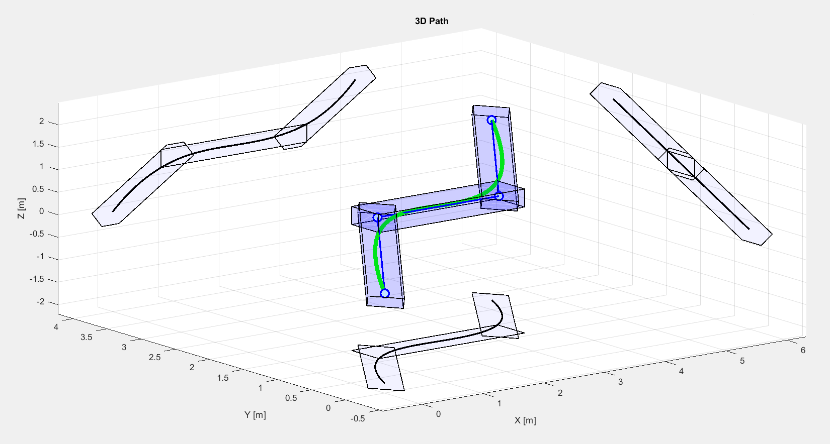
Figure 11.9 Quadrotor flight in 3D (green line) including waypoints/segments (dark blue) and bounding boxes (light blue); also projected onto each dimension.
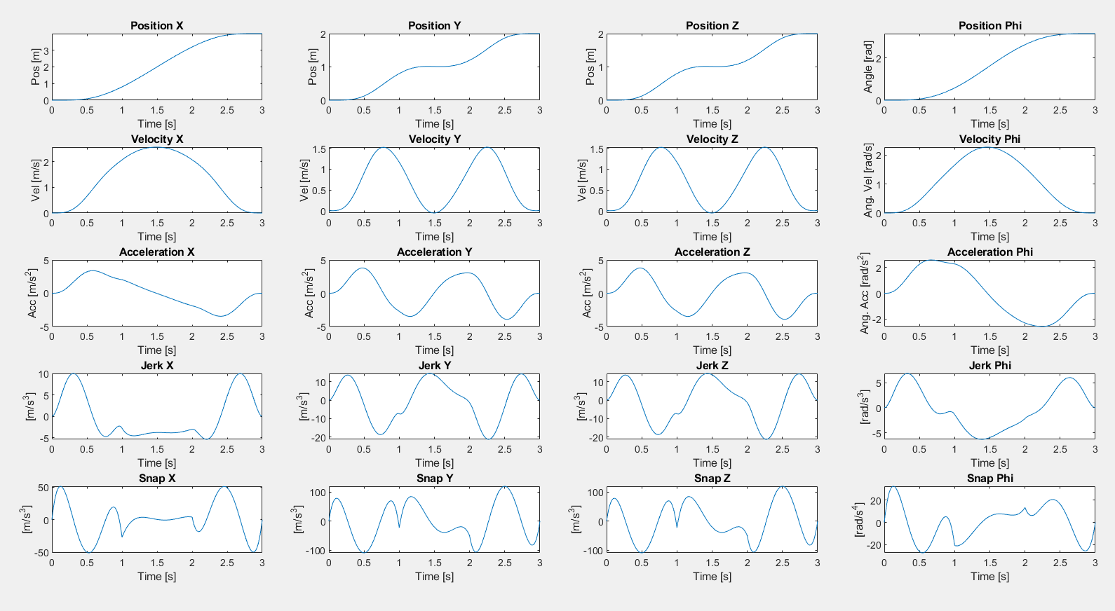
Figure 11.10 Individual trajectories of the quadrotor flight in time for all three dimensions and the angular orientation.