11.8. High-level interface: Basic example
Consider the following linear MPC problem with lower and upper bounds on state and inputs, and a terminal cost term:
This problem is parametric in the initial state \(\color{red} x\) and the first input \(u_0\) is typically applied to the system after a solution has been obtained.
You can download the MATLAB code of this example to try it out for yourself by
clicking here.
11.8.1. Defining the problem data
Let’s define the known data of the MPC problem, i.e. the system matrices \(A\) and \(B\), the prediction horizon \(N\), the stage cost matrices \(Q\) and \(R\), the terminal cost matrix \(P\), and the state and input bounds:
%% system
A = [1.1 1; 0 1];
B = [1; 0.5];
[nx,nu] = size(B);

%% MPC setup
Q = eye(nx);
R = eye(nu);
if( exist('dlqr','file') )
    [~,P] = dlqr(A,B,Q,R);
else
    P = 10*Q;
end
umin = -0.5;     umax = 0.5;
xmin = [-5, -5]; xmax = [5, 5];
11.8.2. Defining the MPC problem
Let’s now dive in right into the problem formulation:
%% FORCESPRO multistage form
% assume variable ordering z(i) = [ui; xi] for i=1...N

% dimensions
model.N     = 11;   % horizon length
model.nvar  = 3;    % number of variables
model.neq   = 2;    % number of equality constraints

% objective
model.objective = @(z) z(1)*R*z(1) + [z(2); z(3)]'*Q*[z(2); z(3)];
model.objectiveN = @(z) [z(2); z(3)]'*P*[z(2); z(3)];

% equalities
model.eq = @(z) [ A(1,:)*[z(2); z(3)] + B(1)*z(1);
                  A(2,:)*[z(2); z(3)] + B(2)*z(1)];

model.E = [zeros(2,1), eye(2)];

% initial state
model.xinitidx = 2:3;

% inequalities
model.lb = [ umin,    xmin  ];
model.ub = [ umax,    xmax  ];
11.8.3. Generating a solver
We have now populated model with the necessary fields to generate a solver
for our problem. Now we use the function FORCES_NLP to generate a solver for
the problem defined by model with the first state as a parameter:
%% Generate FORCESPRO solver

% get options
codeoptions = getOptions('FORCESNLPsolver');
codeoptions.printlevel = 2;
codeoptions.nlp.ad_tool = 'casadi';
%codeoptions.nlp.ad_tool = 'symbolic-math-tbx';

% generate code
FORCES_NLP(model, codeoptions);
11.8.4. Calling the generated solver
Once all parameters have been populated, the MEX interface of the solver can be used to invoke it:
problem.x0 = zeros(model.N*model.nvar,1);
problem.xinit = xinit;
[solverout,exitflag,info] = FORCESNLPsolver(problem);
Tip
Type help solvername to get more information about how to call the solver.
11.8.5. Simulation
Let’s now simulate the closed loop over the prediction horizon \(N\):
%% simulate
x1 = [-4; 2];
kmax = 30;
X = zeros(2,kmax+1); X(:,1) = x1;
U = zeros(1,kmax);
problem.x0 = zeros(model.N*model.nvar,1);
for k = 1:kmax

    problem.xinit = X(:,k);

    [solverout,exitflag,info] = FORCESNLPsolver(problem);

    if( exitflag == 1 )
        U(:,k) = solverout.x01(1);
    else
        error('Some problem in solver');
    end

    %X(:,k+1) = A*X(:,k) + B*U(:,k);
    X(:,k+1) = model.eq( [U(:,k); X(:,k)] )';
end
11.8.6. Results
The results of the simulation are presented in Figure 11.8. The plot on the top shows the system’s states over time, while the plot on the bottom shows the input commands. We can see that all constraints are respected.
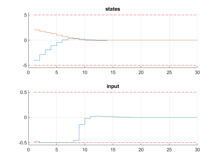
Figure 11.32 Simulation results of the states (top, in blue and red) and input (bottom, in blue) over time. The state and input constraints are plotted in red dashed lines.