11.15. Controlling a crane using a FORCESPRO NLP solver
In this example we will see how to control a crane using the FORCESPRO interior point NLP solver. One interesting feature of this system is that is has a rather large linear subsystem which FORCESPRO can exploit for performance (see Linear subsystem exploitation). The crane is described by the following states:
and the control inputs are given by the voltage rate for the horizontal actuator \(u_{CR}\) and the voltage rate of the rotating actuator \(u_{LR}\). The system dynamics are described by the following ODE:
where \(a_C = \frac{-v_C}{\tau} + \frac{A_C u_C}{\tau}\) and \(a_L = \frac{-v_L}{\tau} + \frac{A_L u_L}{\tau}\) and the constants are given by
For further details on these models we refer to [VukLoock] and [QuirDiehl].
You can download the following MATLAB code of this example to try it out for yourself
by clicking here.
11.15.1. Defining the MPC problem
11.15.1.1. Model dimensions and dynamics
The following code-snippet shows how to define the MPC problem associated with controlling the crane in FORCESPRO. The primal variable of our optimization problem is
%% Define crane model
% Dimensions
model.N     = 20;       % horizon length
model.nvar  = 10;       % number of variables
model.neq   = 8;        % number of equality constraints
model.nh    = 0;        % number of inequality constraint functions
model.npar  = 2;        % number of parameters (these will be the reference values to track)
nx = 8;
nu = 2;

% Dynamics
model.E = [zeros(nx,nu), eye(nx)];
model.continuous_dynamics = @(x,u,p) ode(x,u,p);
Here the right-hand-side of the differential equation ode is defined by the following MATLAB function
function [ dx ] = ode(x,u,~)
    g = 9.81; % gravitational constant
    AC = 0.0474; % gain of GC(s) in m/s/V
    AL = 0.0341; % gain of GL(s) m/s/V
    tau = 0.0247; % time constant of winch dynamics in seconds


    uCR = u(1); % voltage rate for horizontal actuator
    uLR = u(2); % voltage rate for rotating actuator

    xC = x(1); % cart position
    vC = x(2); % cart velocity
    xL = x(3); % cable length
    vL = x(4); % rate of change of cable length
    theta = x(5); % angle of pendulum
    omega = x(6); % rate of change of angle
    uC = x(7); % voltage for horizontal actuator
    uL = x(8); % voltage for rotating actuator

    aT = -(1/tau)*vC + (AC/tau)*uC;
    aL = -(1/tau)*vL + (AL/tau)*uL;

    dx = [  vC; ...
            aT; ...
            vL; ...
            aL; ...
            omega; ...
            -(1/xL)*(aT*cos(theta) + g*sin(theta) + 2*vL*omega); ...
            uCR; ...
            uLR   ];
end
11.15.1.2. System constraints
We put simple constraints on both of the control inputs as well as the voltage for horizontal actuator and the voltage for rotating actuator. We also specify that we have an initial condition for all the states.
% Bounds
model.lb = [ -100, -100, -inf, -inf, -inf, -inf, -inf, -inf, -10, -10 ];
model.ub = [ +100, +100, +inf, +inf, +inf, +inf, +inf, +inf, +10, +10 ];

% Initial state
xinitidx = 3:10;
model.xinitidx = xinitidx;
11.15.1.3. Objective function
The goal of the control will be to track reference values for the cart position and cable length of the crane. Hence, it makes sense to use a Gauss-Newton hessian approximation in our optimization problem. Hence, in FORCESPRO we specify a least squares objective function
% Least squares objective function
model.LSobjective = @(z, p) LScost(z, p);
where the LScost function is defined as follows
function [ r ] = LScost(z,p)
    ep = 1e-5;
    cst = 50;
    sep = sqrt(ep);
    scst = sqrt(cst);
    r = [ sep*z(1); sep*z(2); scst*(z(3)-p(1)); sep*z(4); scst*(z(5)-p(2)); sep*z(6); sep*z(7); sep*z(8); sep*z(9); sep*z(10)];
end
11.15.2. Generating a FORCESPRO interior point NLP solver
In order to generate a solver we first need to choose options to specify the algorithmic specifications (see Solver Options) we want implemented in our solver. The two most important options to mention here is that we specify to use a Gauss-Newton hessian approximation and we want to allow FORCESPRO to exploit linear subsystems of our dynamics.
%% Set codeoptions to specify solver settings
codeoptions = getOptions('CraneSolver');
Ts = 1/100; % sampling time
codeoptions.nlp.integrator.Ts = Ts;
nodes = 4;
codeoptions.nlp.integrator.nodes = nodes;
codeoptions.nlp.integrator.type = 'ERK4';
codeoptions.nlp.integrator.attempt_subsystem_exploitation = 1; % Enable subsystem exploitation for performance
codeoptions.printlevel = 0;
codeoptions.nlp.hessian_approximation = 'gauss-newton';
codeoptions.nlp.ad_tool = 'casadi';

% Generate solver
FORCES_NLP(model, codeoptions);
The last command will generate a FORCESPRO solver which can now be called from MATLAB via the name CraneSolver.
11.15.3. Calling the crane solver
With our FORCESPRO controller at hand we can easily simulate our system in MATLAB as the following code-snippet shows.
%% Simulation
totalTime = 100; % number of seconds
nSamples = totalTime / Ts;

t = 0;
all_refs = zeros(2, nSamples);
cart_data = zeros(2, nSamples);
time = zeros(1, nSamples);
x = [ 0.15; 0; 0.7; 0; 0; 0; 0; 0];
for ii = 1:nSamples

    % get current reference
    ref = getRef(t, totalTime);

    % record data for plotting
    all_refs(:,ii) = ref;
    cart_data(:,ii) = x([1, 3]);
    time(ii) = t;

    % set up problem data
    problem.xinit = x;
    problem.x0 = repmat([0; 0; x],model.N,1);
    problem.all_parameters = repmat(ref,model.N,1);

    % call FORCESPRO solver and check exit status
    [solution, exitflag, info] = CraneSolver(problem);
    if exitflag ~= 1
        error('Encountered solver failure.');
    end

    % extract control and update state
    u = solution.x01(1:2);
    x = RK4( x, u, @(x,u,p) ode(x,u,p), Ts, ref, nodes);
    t = t + Ts;
end
11.15.4. Results
As can be seen from figures Figure 11.47 and Figure 11.48 below the FORCESPRO controller achieves tracking the reference values almost perfectly.
A benchmark running the CraneSolver with and without linear subsystem exploitation on a Raspberry Pi 3 showed an overall reduction of computation time by 22% when exploiting linear subsystems.
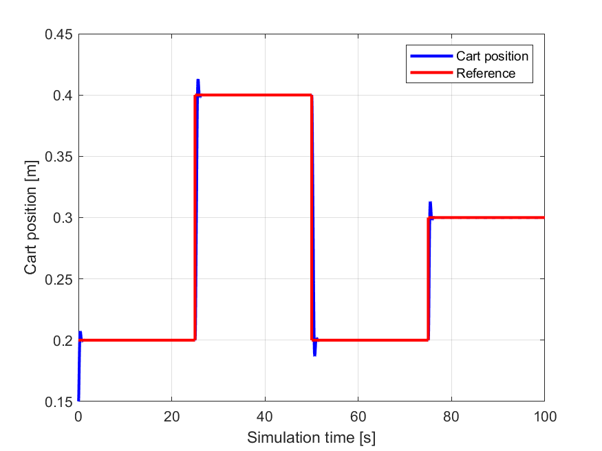
Figure 11.47 The reference values for the cart position (\(x_C\)) seen in red and the simulated cart position seen in blue.
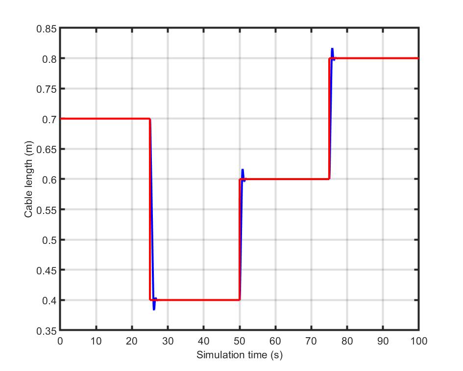
Figure 11.48 The reference values for the cable length (\(x_L\)) seen in red and the simulated cable length seen in blue.
Vukov, Milan & Van Loock, Wannes & Houska, Boris & Ferreau, Joachim & Swevers, Jan & Diehl, Moritz. (2012). Experimental validation of nonlinear MPC on an overhead crane using automatic code generation. Proceedings of the American Control Conference. 6264-6269. 10.1109/ACC.2012.6315390.
Quirynen, Rien & Gros, Sebastien & Diehl, Moritz. (2013). Efficient NMPC for nonlinear models with linear subsystems. Proceedings of the IEEE Conference on Decision and Control. 5101-5106. 10.1109/CDC.2013.6760690.