11.20. High-level interface: Extended optimal EV charging and speed profile example using a 2D motor efficiency map (MATLAB & PYTHON)

This example is an updated and more realistic version of Section 11.19, since it uses 2D motor efficiency map data. In addition to showcasing 2D spline usage, this example also illustrates how to scale optimization variables, which can be used to increase numerical stability of optimization problems in general.

In this example we illustrate the simplicity of the high-level user interface on an optimal electric vehicle (EV) speed and charging management. The controller plans the car’s speed and charging trajectory such that the given route is traversed in the shortest time possible, while simultaneously respecting speed limits as well as vehicle’s and battery’s technical requirements. Furthermore, this example illustrates how to use two-dimensional splines as well as scaling of an optimization problem to make it numerically better conditioned.

11.20.1. Problem Overview

We consider a single EV and a fixed route with given road slopes (i.e. angles) and speed limits. Optionally, some charging stations could be available at predefined locations along the road. Vehicle operation is defined by longitudinal vehicle dynamics, powertrain efficiency and battery capacity. Due to the spatial characteristic of the problem, the formulation is discretized in space domain. This problem is primarily based on the work in [JiaJibItoGor19_2D] and [JiaJibGor20_2D].

11.20.1.1. Vehicle Dynamics

Assuming a sample distance \(L_\mathrm{s}\), the longitudinal velocity of the vehicle in space domain at the discrete step \((i+1)\in\mathcal{I}\) can be determined using the velocity at the previous step \((i)\) and the difference in kinetic energy between these two consecutive steps, as follows:

\[\frac{1}{2}m_\mathrm{eq}\left(v_{i+1}^2 - v_i^2\right) = L_\mathrm{s}\left(F_{\mathrm{t},i} - F_{\mathrm{b},i} - F_{\mathrm{r},i}\right)\]

where the resistance force is comprised of the following three components:

\[F_{\mathrm{r},i} = \underbrace{c_\mathrm{r}m_\mathrm{v}g\cos{(\alpha_\mathrm{i})}}_{\text{rolling resistance}} + \underbrace{m_\mathrm{v}g\sin{(\alpha_\mathrm{i})}}_{\text{gravitational force}} + \underbrace{\frac{1}{2}c_\mathrm{a}A_\mathrm{f}\rho_\mathrm{a}v_i^2}_{\text{air drag force}}\]

The equivalent mass \(m_\mathrm{eq}=m_\mathrm{v}(1 + e_\mathrm{I})\) includes vehicle mass \(m_\mathrm{v}\) and the effect of all rotational masses captured by the mass factor \(e_\mathrm{I}\). The road slope is represented by the road angle \(\alpha\). Variables \(F_\mathrm{t}\geq0\) and \(F_\mathrm{b}\geq0\) represent the traction and braking forces on the wheels, which are generated by the powertrain and mechanical braking system separately (note: regenerative braking capabilities could be included by allowing the traction power to be negative). The total driving resistance \(F_\mathrm{r}\) comprises rolling resistance force, gravitational force and air drag force (while neglecting the direct impact of wind speed), with \(c_\mathrm{a}\) being the air drag coefficient, \(A_\mathrm{f}\) the projected frontal area, \(\rho_\mathrm{a}\) the air density, \(g\) the gravitational acceleration, and \(c_\mathrm{r}\) the rolling resistance coefficient.

The vehicle’s velocity dynamics are thus defined by

\[v_{i+1} = \sqrt{\frac{2\left(F_{\mathrm{t},i} - F_{\mathrm{b},i} - F_{\mathrm{r},i}\right)L_\mathrm{s}}{m_\mathrm{eq}} + v_i^2}\]

with the assumption that the speed is constant while traversing a single discrete road segment. Note that the expression below the square root must be strictly positive in order for the problem to be feasible, as will be discussed later on. In addition to velocity, the time is also a state variable of the model and can be computed as

\[t_{i+1} = t_i + \frac{L_\mathrm{s}}{v_i}\]

11.20.1.2. Vehicle Energetics

EV’s powertrain efficiency \(\eta(v,F_\mathrm{t},\zeta)\) is a function of vehicle’s speed, traction force and battery’s state-of-charge (SoC), as shown by the efficiency maps depicted in Figure 11.73. Nevertheless, the impact of SoC on powertrain efficiency is negligible as SoC does not change dramatically within a short time period if the battery capacity is sufficiently large. Therefore, one could generate several 2D maps of the form \(\eta(v,F_\mathrm{t})\), pre-calculated at different SoC levels such that the most accurate one can be selected according to the current SoC.

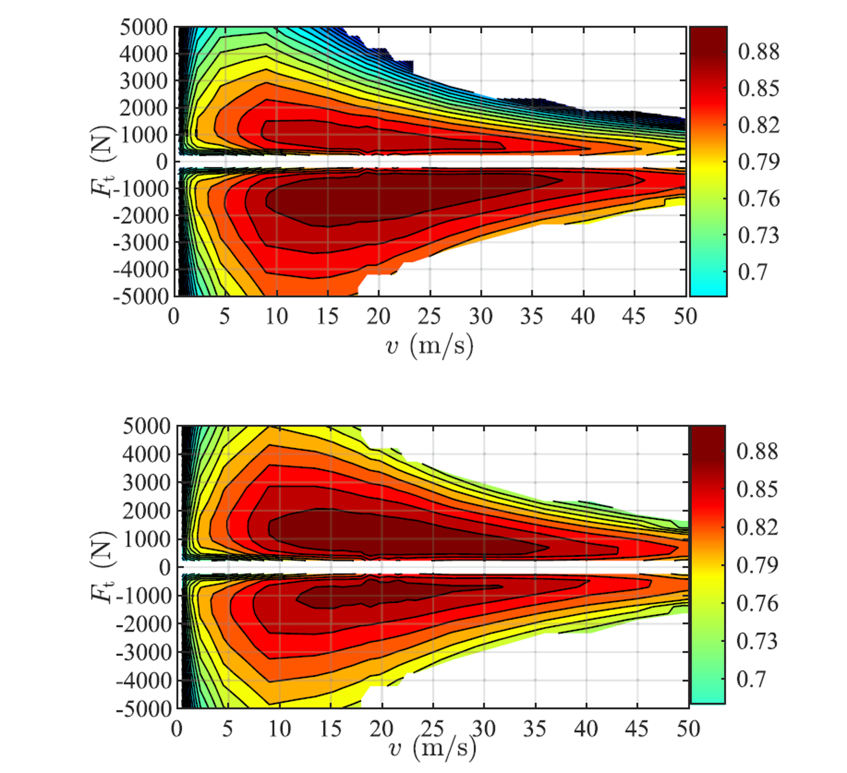
Figure 11.73 2D efficiency maps of the EV’s powertrain with two different SoC levels taken from [JiaJibGor20_2D]: (top) \(\eta\) with SoC \(\zeta=10\,\%\); (bottom) \(\eta\) with SoC \(\zeta=90\,\%\).

For the purpose of this example, we have have generated a single 2D efficiency map depicted in Figure 11.74 used across all SoC levels.

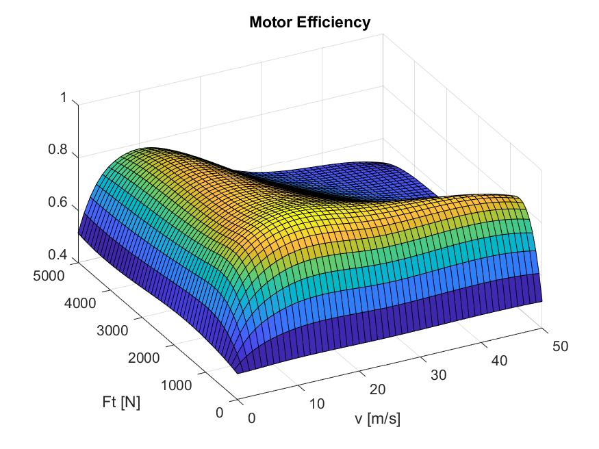
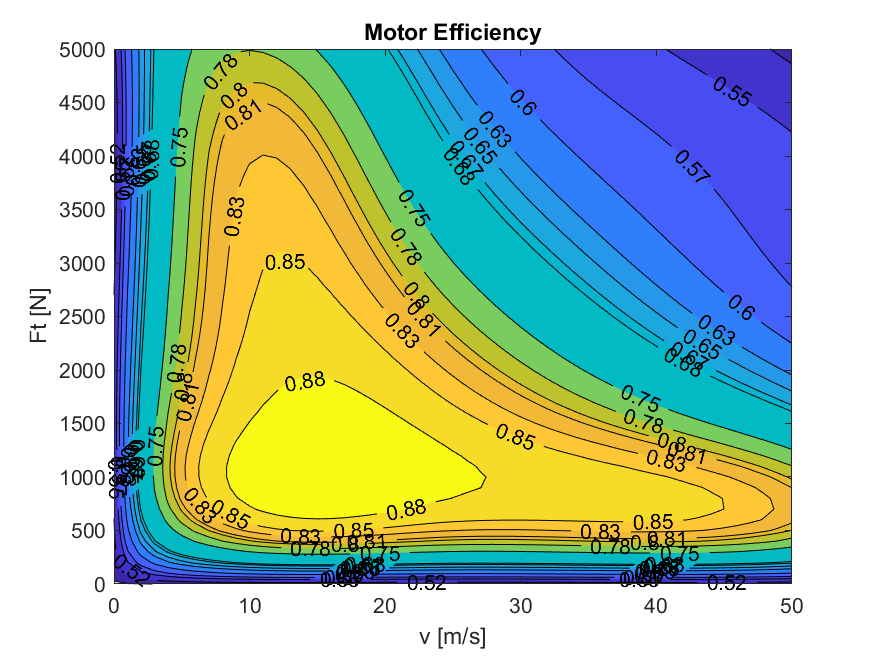
Figure 11.74 Generated 2D EV efficiency map.

In Option 1, we fit the 2D efficiency map \(\eta(v, F_\mathrm{t})\) data as a cubic bivariate spline using Scipy’s SmoothBivariateSpline routine. In order to utilize Scipy’s fitting routines, a valid Python installation needs to be present, even if it is called via MATLAB. Note that not all Python versions are compatible with all MATLAB versions. For a compatibility list see here (Compatibility).

In principle, we could have utilized any of the provided 2D-spline fitting methods. There is one that uses CasADi and does not require a valid Python installation. For an extensive list of the available 2D-spline related methods, see Interpolations 2D (B-splines).

In Option 2, we assume that we have already fitted the 2D-splines (i.e. must be representable as a B-spline) and therefore, we can provide the coefficients matrix in matrix-indexed form (i.e. x corresponds to rows and y corresponds to columns) as well as the knots tx and ty directly.

In this example, we can toggle between the two options by setting useScipy. In MATLAB, the example additionally checks that Python as well as the Python package Scipy are installed using the function validPythonPackages. The Python interface of FORCESPRO already requires a valid Scipy installation, which is why the check is omitted there.

The two 2D-spline options are generated as follows:

MatlabPython

function etaMotorSpline = setupMotorEfficiency()
% Returns a cubic bivariate spline representing motor efficiency as a
% function of velocity and traction force.
%
% The data is taken from "Jia, Y.; Jibrin, R.; Goerges, D.: Energy-Optimal
% Adaptive Cruise Control for Electric Vehicles Based on Linear and
% Nonlinear Model Predictive Control. In: IEEE Transactions on Vehicular
% Technology, vol. 69, no. 12, pp. 14173-14187, Dec. 2020."

    vMaxMEff = 180;     % maximum velocity in the lookup table [km/h]
    FtMaxMEff = 5e3;    % maximum traction force in the lookup table [N]
    vMaxMEff = kmh2ms(vMaxMEff);
    vSampleOrig = 0:vMaxMEff/10:vMaxMEff;
    FtSampleOrig = 0:FtMaxMEff/5:FtMaxMEff;

    % denser grid point selection near the edges with the sharp transitions
    vSampleOrig = [vSampleOrig(1), mean(vSampleOrig(1:2)), vSampleOrig(2:end)];
    FtSampleOrig = [FtSampleOrig(1), mean(FtSampleOrig(1:2)), FtSampleOrig(2:end)];

    %     v [m/s] =        0,  2.5,    5,   10,   15,   20,   25,   30,   35,   40,   45,   50
    etaSampleOrig = [
                        0.50, 0.50, 0.50, 0.50, 0.50, 0.50, 0.50, 0.50, 0.50, 0.50, 0.50, 0.50; ... % F [N] = 0
                        0.50, 0.68, 0.80, 0.85, 0.85, 0.85, 0.85, 0.85, 0.85, 0.85, 0.83, 0.81; ... % F [N] = 500
                        0.50, 0.78, 0.81, 0.88, 0.88, 0.88, 0.88, 0.88, 0.85, 0.83, 0.81, 0.80; ... % F [N] = 1000
                        0.50, 0.75, 0.81, 0.85, 0.88, 0.85, 0.83, 0.81, 0.78, 0.68, 0.65, 0.63; ... % F [N] = 2000
                        0.50, 0.68, 0.80, 0.83, 0.83, 0.81, 0.78, 0.68, 0.65, 0.63, 0.60, 0.57; ... % F [N] = 3000
                        0.50, 0.67, 0.78, 0.81, 0.80, 0.78, 0.65, 0.63, 0.60, 0.57, 0.55, 0.55; ... % F [N] = 4000
                        0.50, 0.67, 0.75, 0.78, 0.75, 0.65, 0.63, 0.60, 0.57, 0.55, 0.52, 0.52; ... % F [N] = 5000
                    ];

    % spline
    useScipy = false;
    if useScipy && validPythonPackages()
        % Option 1: fitting with Scipy's SmoothBivariateSpline
        % convert to 1-D sequences of data points
        [vTemp, FtTemp] = meshgrid(vSampleOrig, FtSampleOrig);
        vSample = reshape(vTemp.', 1, []);
        FtSample = reshape(FtTemp.', 1, []);
        etaSample = reshape(etaSampleOrig', [1, numel(etaSampleOrig)]);

        s = 0.025;
        w = ones(1, length(vSample));
        bbox = [min(vSample), max(vSample), min(FtSample), max(FtSample)];
        kx = 3;
        ky = 3;
        rankTol = 1e-8;
        scaling = [1e1, 1e3, 1];
        etaMotorSpline = ForcesInterpolationFit_SmoothBivariateSpline(vSample, FtSample, etaSample, w, bbox, kx, ky, s, rankTol, scaling);
    else
        % Option 2: providing 2D-spline coefficients
        kx = 3;
        ky = 3;
        tx = [0, 0, 0, 0, 6.3993742001266, 24.1805094335686, 50, 50, 50, 50];
        ty = [0, 0, 0, 0, 760.320551795358, 1503.23831410745, 5000, 5000, 5000, 5000];
        coeffs = [0.498727471092637   0.511037494098402   0.524901875945660   0.548511907792580   0.475607487652389   0.513135686437586
                  0.498465143841756   0.654046675851965   0.783006359203673   0.713858506960411   0.676705972846789   0.681154627267599
                  0.510442836827170   0.854158083414314   1.007125597517271   0.847628255554849   1.018658592375758   0.878826758082995
                  0.495093430686428   0.735511289747710   0.857756122056489   0.863078750613390   0.548595365620131   0.497927393614425
                  0.510240152112442   0.835399001169469   0.952683895958243   0.536982511482952   0.563982968586042   0.577416237725016
                  0.501474795696226   0.773879473939183   0.878143062979889   0.444534437467682   0.615960539904494   0.508404545245928];
        etaMotorSpline = ForcesInterpolation2D(tx, ty, coeffs, kx, ky);
    end
end

Note that for the fitting you can set a scaling vector for numerically robustifying Scipy’s 2D spline fitting routine in case the input and output variables have vastly different magnitudes. The returned spline takes care of scaling such that the inputs to the spline are still the physical (unscaled) quantities. This scaling is solely utilized for the spline fitting and is different from optimization variable scaling, which follows later in this example (see Section 11.20.2.1).

Assuming a set of predefined charging stops at discrete spatial steps \(k\in\mathcal{K}\subset\mathcal{I}\), we can include either optional or mandatory charging at each of those stops (to be defined by the user). Given the implemented powertrain efficiency \(\eta_i(F_{\mathrm{t},i})\) and potential charging decisions, the driving energy depletion and charging instances are incorporated into the SoC dynamics at discrete step \(i\) as:

\[\zeta_{i+1} = \zeta_i - \frac{F_{\mathrm{t},i} L_\mathrm{s}}{\eta_i E_\mathrm{cap}} + \frac{P_{\mathrm{ch},i}}{E_\mathrm{cap}} \Delta t_i\]

where \(E_\mathrm{cap}\) denotes the battery’s energy capacity, \(P_{\mathrm{ch},i}(\zeta_i)\) is a vehicle’s charging power dependent on the SoC, and \(\Delta t_i\) is the total charging time spent at location \(i\in\mathcal{K}\). Note that SoC \(\zeta\) is normalized on an interval \([0,1]\).

In this example we will particularly focus on the performance of a BMW i3. The charging profiles \(P_\mathrm{ch}(\zeta)\) for three production models with different battery capacities are depicted in Figure 11.75 [Fastned_2D], and can be approximated by a piecewise-affine function as shown in Figure 11.76.

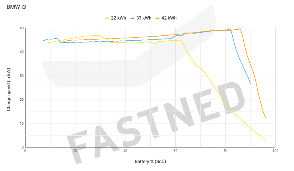
Figure 11.75 Actual charging profile of BMW i3 as a function of vehicle’s SoC.

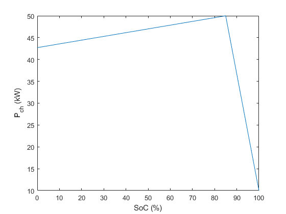
Figure 11.76 Implemented piecewise-affine charging profile for the \(42\,\mathrm{kWh}\) vehicle as a function of vehicle’s SoC.

The code for computing the \(P_\mathrm{ch}(\zeta)\) spline function is given below. Note that the Python implementation uses a shape-preserving piecewise-cubic representation instead of piecewise-linear one.

MatlabPython

function Pch = setupChargingPower(PchMax)
% Returns piecewise linear representation of charging power as a
% function of vehicle's SoC.
%
% The data is taken from Fastned charging chart available at
% https://support.fastned.nl/hc/en-gb/articles/204784718-Charging-with-a-BMW-i3
%
% NOTE: Python example uses shape-preserving piecewise cubic spline
% approximation ('pchip') which might lead to negligible result
% discrepancies between the two clients when directly compared.
    socSample = [0.15, 0.85, 1.0];
    PchSample = [0.88, 1, 0.2]*PchMax;
    Pch = ForcesInterpolationFit(socSample,PchSample,'linear');
end

Clearly, the time dynamics would have to be modified as well:

\[t_{i+1} = t_i + \frac{L_\mathrm{s}}{v_i} + \Delta t_i\]

with \(\Delta t_i\approx 0\) for all non-charging spatial steps \(i\notin\mathcal{K}\), and \(v_i\approx \underline{v}\) for all charging spatial steps \(i\in\mathcal{K}\), with \(\underline{v}>0\) being th lower speed bound. The latter is not set to zero for two reasons: 1) it would lead to infeasibility due to \(v_i\) being in the denominator; 2) it reflects the average speed across the distance \(L_s\), which includes both the driving and the charging instances, and is therefore greater than zero. This implies that the final vehicle model comprises three states \(x=[v,t,\zeta]^\top\) and three control inputs \(u=[F_\mathrm{t},F_\mathrm{b},\Delta t]^\top\), with the model dynamics described by

\[\begin{split}v_{i+1} &= \sqrt{\frac{2\left(F_{\mathrm{t},i} - F_{\mathrm{b},i} - F_{\mathrm{r},i}\right)L_\mathrm{s}}{m_\mathrm{eq}} + v_i^2} \\ t_{i+1} &= t_i + \frac{L_\mathrm{s}}{v_i} + \Delta t_i \\ \zeta_{i+1} &= \zeta_i - \frac{F_{\mathrm{t},i} L_\mathrm{s}}{\eta_i E_\mathrm{cap}} + \frac{P_{\mathrm{ch},i}}{E_\mathrm{cap}} \Delta t_i\end{split}\]

Additionally, we will include a slack variable \(s\geq0\) into control vector \(u\), as it is used to relax the upper and lower bounds on vehicle’s SoC.

11.20.1.3. Bounds

In terms of bounds on state variables, we impose upper and lower limits on vehicle’s velocity and SoC, dictated by the road speed limits and battery specifications:

\[\begin{split}\underline{v} &\leq v_i \leq \bar{v}_i \\ \underline{\zeta} - s_i &\leq \zeta_i \leq \bar{\zeta} + s_i\end{split}\]

The upper speed bound \(\bar{v}_i\) is stage-dependent, dictated by the spatial discretization of the road speed limits, whereas the lower speed bound \(\underline{v}\) is kept constant across all stages. For charging instances \(i\in\mathcal{K}\), the upper speed bound can optionally be set to \(\bar{v}_i\approx\underline{v}\), indicating that the vehicle has to reduce speed. The SoC limits \(\underline{\zeta}\) and \(\bar{\zeta}\) are also stage independent and implemented as soft bounds.

All control variables are nonnegative and upper bounded with appropriate physical and technical limits:

\[\begin{split}0 &\leq \Delta t_i \leq \overline{\Delta t}_i \\ 0 &\leq F_{\mathrm{t},i} \leq \overline{F}_{\mathrm{t},i} \\ 0 &\leq F_{\mathrm{b},i} \leq \overline{F}_\mathrm{b} \\\end{split}\]

Here, \(\overline{\Delta t}_i\) denotes maximum permissible charging time and is set to \(\overline{\Delta t}_i\approx 0, \forall i\notin\mathcal{K}\), whereas \(\overline{F}_{\mathrm{t},i}\) and \(\overline{F}_\mathrm{b}\) are vehicle’s physical upper bounds on maximum traction and breaking force, respectively. Note that the traction force limit is comprised of the constant friction limit \(\overline{F}_{\mathrm{t}}\) and the hyperbolic traction function of vehicle’s velocity \(\overline{F}_{\mathrm{t},i}^\mathrm{hyp}(v_i)\), i.e.

\[\overline{F}_{\mathrm{t},i} = \min\left(\overline{F}_{\mathrm{t}}, \overline{F}_{\mathrm{t},i}^\mathrm{hyp}(v_i)\right)\]

as depicted in Figure 11.77. The actual function implemented in this example is showcased in Figure 11.78.

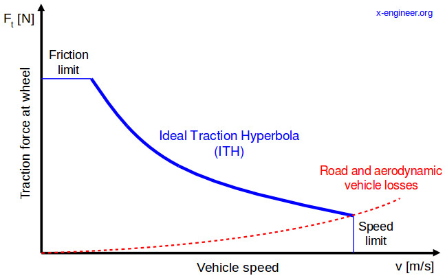
Figure 11.77 Maximum permissible traction force as a function of vehicle’s velocity taken from [xEngineer_2D].

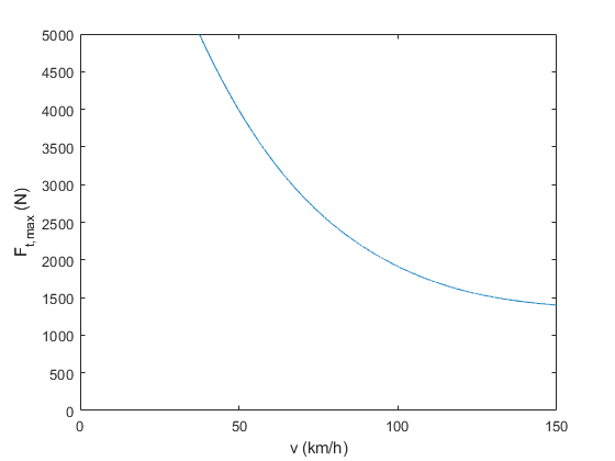
Figure 11.78 Implemented traction force hyperbola as a function of vehicle’s velocity.

The computation of ideal traction hyperbola \(\overline{F}_\mathrm{t,hyp}(v)\) in the cubic spline form is provided below.

MatlabPython

function FtMaxHypSpline = setupTractionForceHyperbola(vMax,FtMax)
% Returns cubic spline representing maximum traction force as a function of
% vehicle's speed
%
% The data is generated based on the technical article provided at
% https://x-engineer.org/need-gears/
    vSample = [0.25, 0.4, 0.6, 0.8, 1.0]*vMax;
    FtMaxHypSample = [1.0, 0.67, 0.43, 0.32, 0.28]*FtMax;
    FtMaxHypSpline = ForcesInterpolationFit(vSample,FtMaxHypSample);
end

11.20.1.4. MPC Formulation

A complete MPC problem formulation can thus be described as follows:

\begin{align*} \text{minimize} \quad & t_N + \sum_{i=0}^{N-1} \left(\omega_\mathrm{s} s_i + \omega_\mathrm{e} F_{\mathrm{t},i}^2 + \omega_\mathrm{b} F_{\mathrm{b},i}^2 \right) \\ \text{subject to} \quad & v_{i+1} = \sqrt{\frac{2L_\mathrm{s}}{m_\mathrm{eq}}\left(F_{\mathrm{t},i} - F_{\mathrm{b},i} - F_{\mathrm{r},i}\right) + v_i^2} \\ & t_{i+1} = t_i + L_\mathrm{s}v_i^{-1} + \Delta t_i \\ & \zeta_{i+1} = \zeta_i - \frac{L_\mathrm{s}}{\eta_i E_\mathrm{cap}}F_{\mathrm{t},i} + \frac{P_{\mathrm{ch},i}}{E_\mathrm{cap}} \Delta t_i \\ & \underline{v} \leq v_i \leq \bar{v}_i \\ & \underline{\zeta} - s_i \leq \zeta_i \leq \bar{\zeta} + s_i \\ & 0 \leq \Delta t_i \leq \overline{\Delta t}_i \\ & 0 \leq F_{\mathrm{t},i} \leq \overline{F}_{\mathrm{t},i} \\ & 0 \leq F_{\mathrm{b},i} \leq \overline{F}_\mathrm{b} \\ & 0 \leq s_i \\ & x_0 = x_\mathrm{init} \end{align*}

with the objective function explained in detail in the subsequent sections.

11.20.1.5. Model Parameters

As stated previously, in this example we focus on a highest energy capacity model of BMW i3, defined by the following parameters obtained from [BMWi3_2D]:

\begin{align*} m_\mathrm{v} &= 1345\,\mathrm{kg} \\ e_\mathrm{I} &= 1.06 \\ A_\mathrm{f} &= 2.38\,\mathrm{m^2} \\ \rho_\mathrm{a} &= 1.206\,\mathrm{kg/m^3} \\ c_\mathrm{a} &= 0.29 \\ c_\mathrm{r} &= 0.01 \\ \overline{F}_\mathrm{t} &= 5\,\mathrm{kN} \\ \overline{F}_\mathrm{b} &= 10\,\mathrm{kN} \\ E_\mathrm{cap} &= 37.9\,\mathrm{kWh} \\ \bar{P}_\mathrm{ch} &= 50\,\mathrm{kW} \\ \underline{v} &= 30\,\mathrm{km/h} \\ \bar{v} &= 180\,\mathrm{km/h} \\ \underline{\zeta} &= 0.1 \\ \bar{\zeta} &= 0.9 \\ \end{align*}

MatlabPython

function param = defineVehicleParameters(trip)
% Returns vehicle parameters
    %% Constant vehicle parameters (not to be changed)
    % The data is obtained from "Technical specifications of the BMW i3
    % (120 Ah)" valid from 11/2018 and available at
    % https://www.press.bmwgroup.com/global/article/detail/T0285608EN/

    % Gravitational acceleration (m/s^2)
    param.g = 9.81;
    % Vehicle mass (kg)
    param.mv = 1345;
    % Mass factor (-)
    param.eI = 1.06;
    % Equivalent mass (kg)
    param.meq = (1+param.eI)*param.mv;
    % Projected frontal area (m^2)
    param.Af = 2.38;
    % Air density (kg/m^3)
    param.rhoa = 1.206;
    % Air drag coefficient (-)
    param.ca = 0.29;
    % Rolling resistance coefficient (-)
    param.cr = 0.01;
    % Maximum traction force (N)
    param.FtMax = 5e3;
    % Minimum traction force (N)
    param.FtMin = 0;
    % param.FtMin = -1.11e3;
    % Maximum breaking force (N)
    param.FbMax = 10e3;
    % Battery's energy capacity (Wh)
    % BMW i3 60Ah - 18.2kWh; BMW i3 94Ah - 27.2kWh; BMW i3 120Ah - 37.9kWh
    param.Ecap = 37.9e3;
    % Maximum permissible charging time (s)
    param.TchMax = 3600;
    % Charging power (W)
    % 7.4 kW on-board charger on IEC Combo AC, optional 50 kW Combo DC
    param.PchMax = 50e3;
    % Power dissipation factor (-) (adjusted for Munich - Cologne trip in
    % order to achieve realistic BMW i3 range of ~260km
    if trip.type == 1
        param.pf = 1;
    else
        param.pf = 0.4;
    end
    % Minimum vehicle velocity (km/h)
    param.vMin = 30;
    % Maximum vehicle velocity (km/h)
    param.vMax = 150;
    % Minimum SoC (-)
    param.SoCmin = 0.1;
    % Maximum SoC (-)
    param.SoCmax = 0.9;

    %% Variable vehicle parameters
    % Motor efficiency (-)
    param.eta = setupMotorEfficiency();
    % Charging power (W)
    param.Pch = setupChargingPower(param.PchMax);
    % Traction force hyperbola (upper limit) (N)
    param.FtMaxHyp = setupTractionForceHyperbola(kmh2ms(param.vMax), param.FtMax);
end

Trip parameters are defined by the user. Here we focus on two benchmark studies: 1) a \(50\,\mathrm{km}\) long trip with five EV charging stations and low initial SoC; and 2) an actual \(573\,\mathrm{km}\) long Munich - Cologne trip with four EV charging stations and fully charged vehicle.

MatlabPython

% Trip parameters (provided by the user)
% Note: Accuracy and feasibility of the solution are not guaranteed when
% the `trip.reduceSpeed` flag is disabled due to inherent mixed-integer
% nature of the problem!

% Trip type (0 - long (Munich - Cologne); 1 - short)
trip.type = 1;

if trip.type == 1
    % Spatial discretization step (km)
    trip.Ls = 1;
    % Trip distance (km)
    trip.dist = 50;
    % EV charging station locations (km)
    trip.kmPosCh = [8, 18, 30, 40, 45];
    % Force vehicle to reduce speed at charging locations (1 - yes; 0 - no)
    trip.reduceSpeed = 0;
    % Initial vehicle speed (km/h)
    trip.initSpeed = 30;
    % Initial SoC [0, 1]
    trip.initSoC = 0.35;
elseif trip.type == 0
    % Spatial discretization step (km)
    trip.Ls = 1;
    % Trip distance (km)
    trip.dist = 573;
    % EV charging station locations (km)
    trip.kmPosCh = [110, 150, 250, 375];
    % Force vehicle to reduce speed at charging locations (1 - yes; 0 - no)
    trip.reduceSpeed = 1;
    % Initial vehicle speed (km/h)
    trip.initSpeed = 30;
    % Initial SoC [0, 1]
    trip.initSoC = 0.9;
else
    error('Incorrect input: trip type should be either 0 or 1.');
end

You can download the code of this example to try it out for yourself by clicking here (MATLAB) or here (Python).

11.20.2. Defining the MPC Problem

11.20.2.1. Scaling

Since the physical quantities of this example (e.g. SoC or traction force) have vastly different magnitudes, it is a numerically sensitive optimization problem. Hence, we utilize scaling to keep the optimization variables (i.e. scaled down physical quantities) in a similar range numerically. It is enough to approximately set the scaling vector equal to the order of magnitudes of the physical states and inputs. For this purpose we define a scaling vector, which will be constant throughout the example:

MatlabPython

% Assume variable ordering zi = [u{i}; x{i}] for i=1...N
% zi = [slack(i); Ft(i); Fb(i); deltaTch(i); v(i); t(i); SoC(i)]
% pi = [vMax(i); vMin(i); alpha(i); TchMax(i); Ls(k)] #k - iteration No.

%% Scaling Vector
% Scaling factors approximately set equal to order of magnitude of
% the corresponding physical states and inputs
scalingVec = [1, 1e4, 1e4, 1e4, 1e2, 1e4, 1].';

11.20.2.2. Objective function

The primary goal is to minimize the total driving time, i.e. minimize terminal variable \(t_N\) at the last stage \(i=N\):

\[f(z, p_N) = z(6)\]

In addition, we want to minimize the stage cost associated with slack variable \(s, \forall i\in\mathcal{I}\):

\[f(z, p_i) = \omega_\mathrm{s} z(1)\]

where \(\omega_\mathrm{s}\) is an appropriately high weight factor.

Optionally, one could opt for ensuring comfortable driving operation and pursuing energy economy improvements. In such case, additional terms could be included in the stage cost function, e.g.

\[f(z, p_i) = \omega_\mathrm{s} z(1) + \omega_\mathrm{e} z(2)^2 + \omega_\mathrm{b} z(3)^2\]

The second term imposes a penalty on consumed energy during driving by reducing the applied traction force, whereas the third term minimizes the total braking force. The corresponding weight factors \(\omega_\mathrm{e}\) and \(\omega_\mathrm{b}\) provide a trade-off between different objectives. Furthermore, one could also penalize jerking, i.e. a change in the traction force between consecutive steps, using another slack variable.

In the code, we scale the optimization variables back to their physical values before multiplying them with the cost weightings. At the end, we scale down the entire cost down again by a scalar costScaling factor in order to have limited cost magnitudes. We could have also omitted the scaling back up to the physical quantities in the cost function by choosing different cost weighting factors. The cost functions are coded in MATLAB and Python as follows:

MatlabPython

% Objective function
costScaling = 1e3;
model.objective = @(z) objective(z, scalingVec, costScaling);
model.objectiveN = @(z) objectiveN(z, scalingVec, costScaling);

function [stageCost] = objective(z, scalingVec, costScaling)
    z = z.*scalingVec;

    R = [ 1e-7,  0;
          0,    1e-6];
    slackCostFactor = 1e6;
    stageCost = slackCostFactor*z(1) + [z(2);z(3)]'*R*[z(2);z(3)];

    stageCost = stageCost/costScaling;
end

function [terminalCost] = objectiveN(z, scalingVec, costScaling)
    z = z.*scalingVec;

    terminalCost = z(6);

    terminalCost = terminalCost/costScaling;
end

11.20.2.3. Equality constraints

The equality constraints model.eq in this example results from the vehicle’s dynamics and energetics model given above. Importantly, we have to scale back up the optimization variables to the physical quantities at the very beginning of the function. With the physical quantities we calculate the dynamics equation as usual and then we scale back down the next state (or state derivative in case of continuous dynamics). Note that we are using the fitted 2D-spline in the dynamics equation for the SoC. The code is implemented as follows:

MatlabPython

% Problem dimensions
nx = 3;
nu = 4;
np = 5;
nh = 7;

model.N = round(trip.dist/trip.Ls); % horizon length
if mod(model.N,1)~=0
    error('Incorrect input: trip distance should be an exact multiple of the spatial discretization step.');
end
model.nvar = nx + nu;               % number of variables
model.neq  = nx;                    % number of equality constraints
model.nh   = nh;                    % number of inequality constraints
model.npar = np;                    % number of runtime parameters

% Dynamics, i.e. equality constraints
model.eq = @(z,p) dynamics(z, p, param, scalingVec, nu, nx);

model.E = [zeros(nx,nu),eye(nx)];

% Initial and final conditions
model.xinitidx = nu+1:nu+nx;

function [xNext] = dynamics(z, p, param, scalingVec, nu, nx)
    z = z.*scalingVec;

    xNext = [sqrt(ForcesMax(2*p(5)/param.meq*(z(2) - z(3) - param.cr*param.mv*param.g*cos(p(3)) - param.mv*param.g*sin(p(3)) - 0.5*param.ca*param.Af*param.rhoa*z(5)^2) + z(5)^2, 1e-5));
            z(6) + p(5)/z(5) + z(4);
            z(7) - param.pf*p(5)*z(2)/(3600*param.eta(z(5), z(2))*param.Ecap) + param.Pch(z(7))*z(4)/(3600*param.Ecap)];

    xNext = xNext./scalingVec(nu+1:nu+nx);
end

The use of smooth maximum approximation (see section Section 19.3) ensures a positive square root term and thus a feasible solution.

11.20.2.4. Inequality constraints

Since our optimization variables are scaled, it is crucial to scale down the physical box-bound constraints.

The nonlinear inequality constraints model.ineq comprise all decision variable bounds described previously. For the nonlinear inequality constraints, we scale back up the optimization variables to physical quantities and define the physical constraints as usual. Optionally, we scale down again the entire nonlinear constraints by their approximate order of magnitudes for additional numerical stability. We keep in mind that if the bounds of the nonlinear inequality constraints model.hl and model.hu were not -inf or 0, they would have been affected by the scaling as well. For purposes of model feasibility, two additional trivial constraints pertaining to the vehicle velocity’s square root term are included in the model, as shown in the code-snippets.

MatlabPython

% Inequality constraints
% Upper/lower variable bounds lb <= z <= ub
%                             inputs                       |                states
%           slack       Ft       Fb            Tch                     v           t      SoC
model.lb = [0,     param.FtMin,  0.,           0.,            kmh2ms(param.vMin),  0.,    0.]./scalingVec.';
model.ub = [0.1,   param.FtMax,  param.FbMax,  param.TchMax,  kmh2ms(param.vMax),  +inf,  1.]./scalingVec.';

% Nonlinear inequalities hl <= h(z,p) <= hu
model.ineq = @(z,p) ineq(z, p, param, scalingVec);

% Upper/lower bounds for inequalities
model.hu = [0,    0,    0,    0,    0,    0];
model.hl = [-inf, -inf, -inf, -inf, -inf, -inf];

function [h] = ineq(z, p, param, scalingVec)
    z = z.*scalingVec;

    h = [z(2) - param.FtMaxHyp(z(5));
        z(4) - p(4);
        z(7) - param.SoCmax - z(1);
        param.SoCmin - z(7) - z(1);
        2*p(5)/param.meq*(z(2) - z(3) - param.cr*param.mv*param.g*cos(p(3)) - param.mv*param.g*sin(p(3)) - 0.5*param.ca*param.Af*param.rhoa*z(5)^2) + z(5)^2 - kmh2ms(ForcesMax((1-z(4))*p(1), param.vMin+1))^2;
        kmh2ms(p(2))^2 - (2*p(5)/param.meq*(z(2) - z(3) - param.cr*param.mv*param.g*cos(p(3)) - param.mv*param.g*sin(p(3)) - 0.5*param.ca*param.Af*param.rhoa*z(5)^2) + z(5)^2)];

    h = h./[scalingVec(2); scalingVec(4); scalingVec(7); scalingVec(7); scalingVec(5); scalingVec(5)];
end

11.20.2.5. Generating the FORCESPRO NLP solver

To generate a suitable NLP solver for our MPC problem one needs to provide the model and codeoptions. The model has been populated above and we now specify the desired codeoptions and generate the solver by calling FORCES_NLP. Importantly, in order to use the provided 2D-spline functionality, the automatic differentiation tool must be CasADi. Furthermore, the CasADi 2D-splines require the usage of MX CasADi-variables, which can be set in the codeoptions. The following code-snippets show how this can be done:

MatlabPython

% Generate FORCESPRO solver

% Define solver options
codeoptions = getOptions('FORCESNLPsolver');
codeoptions.printlevel = 0;
codeoptions.nlp.compact_code = 1;
codeoptions.maxit = 300

% 2D-splines require the MX CasADi variables
codeoptions.nlp.ad_expression_class = 'MX'

% Generate code
FORCES_NLP(model, codeoptions);

11.20.2.6. Calling the solver

Once the solver has been generated it needs to be provided with initial and runtime parameters. Importantly, we need to scale down the physical initial state and scale back up the FORCESPRO solution to the physical quantities. If a physically valid trajectory would be utilized as an initial guess, we would need to scale the initial guess down as well. Here we use \(0\) as initial guess for simplicity’s sake. In this example we are running a single full-horizon snapshot instead of a traditional rolling-horizon MPC, as follows:

MatlabPython

function sim = runSimulation(trip, param, model)
% Defines initial and stage-dependent runtime parameters and solves the
% problem
    problem.x0 = zeros(model.N*model.nvar,1);
    kMax = model.N;
    np = model.npar;

    %% Initialize system states
    if trip.initSpeed < param.vMin || trip.initSpeed > param.vMax
        v1 = kmh2ms(param.vMin);
        warning('Initial vehicle speed is outside of the speed limits. It will be set to the minimum speed limit at t=0.')
    else
        v1 = kmh2ms(trip.initSpeed);
    end

    if trip.initSoC < param.SoCmin || trip.initSoC > param.SoCmax
        SoC1 = 0.5;
        warning('Initial vehicle state-of-charge is outside of the limits. It will be set to 50% at t=0.')
    else
        SoC1 = trip.initSoC;
    end

    % Initialize the problem
    % X(1) = [v(1); t(1); SoC(1)]
    problem.xinit = [v1; 0; SoC1]./scalingVec(nu+1:nu+nx);

    %% Define spatially distributed (i.e. stage-dependent) parameters
    % Road speed limits and slope angles
    [vMaxRoad, ~, vMinRoad, alpha] = setupRoadParameters(param.vMin, trip);

    % Maximum permissible charging time
    deltaTchMax = setupChargingTime(param.TchMax, trip);

    % Set runtime parameters
    problem.all_parameters = zeros(np*model.N,1);
    for i = 1:model.N
        problem.all_parameters((i-1)*np+1:i*np) = [vMaxRoad(i); vMinRoad(i); alpha(i); deltaTchMax(i); trip.Ls*1e3];
    end

    %% Solve the problem
    [solverout,exitflag,info] = FORCESNLPsolver(problem);
    sim.exitflag = exitflag;

    if exitflag == 1
        sim.Z = unpackStruct(solverout,model.nvar).*scalingVec.';
        sim.kMax = kMax;
        sim.solvetime = info.solvetime;
        sim.iters = info.it;
        sim = displayResults(sim);
    else
        error('Some problem in solver.');
    end
end

11.20.2.7. Results

We consider two trips of different lengths previously described in section Section 11.20.1.5 with three benchmark studies conducted for the shorter trip and two studies for the longer trip:

1. a short trip of \(50\,\mathrm{km}\) with arbitrarily generated road profile, \(5\) charging stations along the road, and vehicle’s initial SoC of: a) \(75\,\%\); b) \(50\,\%\); and c) \(25\,\%\).

2. a long trip of \(573\,\mathrm{km}\) representing a Munich - Cologne trip with actual road profile, vehicle’s initial SoC of \(90\,\%\), and: a) \(4\) charging stations along the road; and b) \(2\) charging stations along the road.

Studies 1a - 1c have the same allocation of charging stations, with chargers placed at \(8\,\mathrm{km}\), \(18\,\mathrm{km}\), \(30\,\mathrm{km}\), \(40\,\mathrm{km}\) and \(45\,\mathrm{km}\) marks. Furthermore, we allow optional charging for all three studies. On the other hand, a Munich - Cologne trip 2a considers four chargers placed at \(110\,\mathrm{km}\), \(150\,\mathrm{km}\), \(250\,\mathrm{km}\) and \(375\,\mathrm{km}\), while trip 2b has two available chargers at \(150\,\mathrm{km}\) and \(375\,\mathrm{km}\). In contrast to the short trip, here we impose mandatory charging requirement. The most notable trip metrics for all five studies are showcased in Table 11.2.

Table 11.2 Summary of vehicle performance for different trip parameters and initial SoC levels.

Trip	Distance	SoC (t=0)	# stations	# stops	Total time	Charge time
1a	50 km	75 %	5	0	33.75 min	0 min
1b	50 km	50 %	5	1	37.75 min	2.36 min
1c	50 km	25 %	5	3	53.56 min	15.21 min
2a	573 km	90 %	4	4	351.34 min	71.79 min
2b	573 km	90 %	2	2	354.30 min	72.02 min

The simulation results for studies 1a and 1b are depicted in Figure 11.79 and Figure 11.80, respectively. Since the vehicle has sufficiently high SoC, no charging is needed in first case and only a tiny amount of charging is required in the latter case. However, in the second trip the vehicle is forced to reduce its velocity below the speed limit in order to preserve energy and complete the trip with sufficient battery charge, which leads to a higher trip time.

A low initial SoC in study 1c forces the vehicle to charge, as shown in Figure 11.81, which leads to drastically higher trip time. The EV decides to stop at first three charging stops and charge just enough to complete the trip with the SoC at the lower bound.

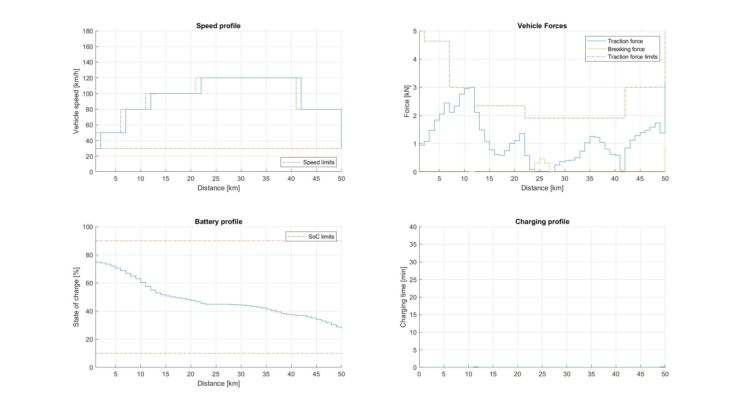
Figure 11.79 Vehicle performance on a short trip with 5 charging stations and 75 % initial SoC.

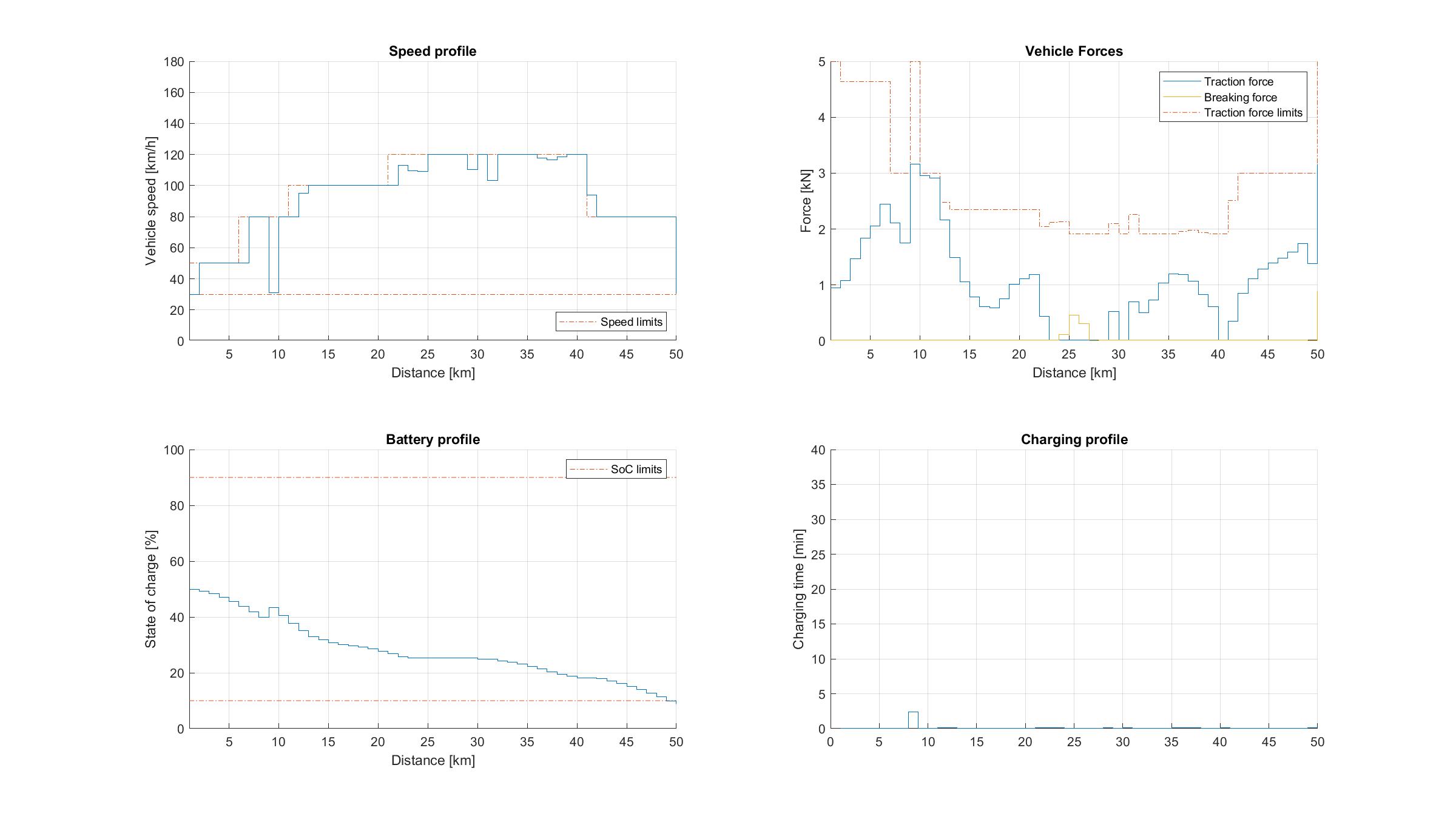
Figure 11.80 Vehicle performance on a short trip with 5 charging stations and 50 % initial SoC.

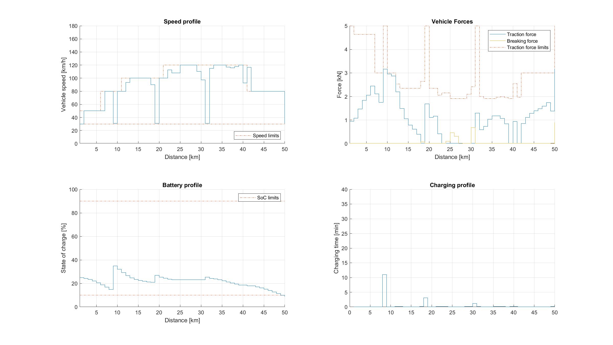
Figure 11.81 Vehicle performance on a short trip with 5 charging stations and 25 % initial SoC.

The longer trip studies with mandatory charging presented in Figure 11.82 and Figure 11.83 again indicate that the EV will complete the trip at the minimum permissible SoC in order to minimize the total charging time. The results also suggest that the vehicle will intentionally reduce speed in order to preserve energy, thus achieving a trade-off between driving and charging time. The availability of only 2 chargers in study 2b forces the vehicle to drastically reduce speed midway through the trip.

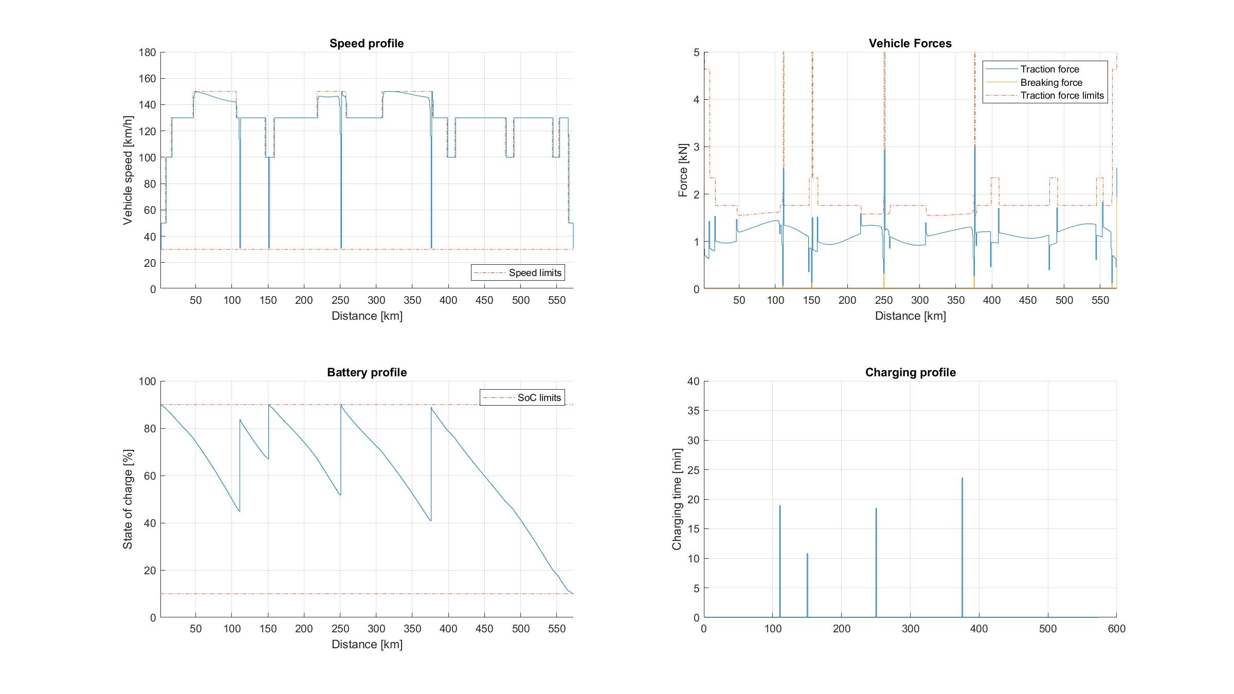
Figure 11.82 Vehicle performance on a long trip with 4 charging stations and 90 % initial SoC.

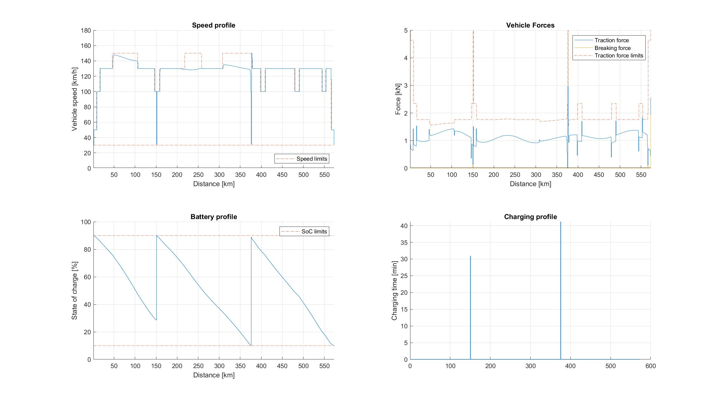
Figure 11.83 Vehicle performance on a long trip with 2 charging stations and 90 % initial SoC.

[JiaJibItoGor19_2D]

Jia Y.; Jibrin, R.; Itoh Y.; Görges, D.: Energy-Optimal Adaptive Cruise Control for Electric Vehicles in Both Time and Space Domain based on Model Predictive Control. In: IFAC-PapersOnLine, vol. 50, no. 2, 2017, pp. 13-20, 2019.

[JiaJibGor20_2D]

Jia, Y.; Jibrin, R.; Görges, D.: Energy-Optimal Adaptive Cruise Control for Electric Vehicles Based on Linear and Nonlinear Model Predictive Control. In: IEEE Transactions on Vehicular Technology, vol. 69, no. 12, pp. 14173-14187, Dec. 2020.

[Fastned_2D]

Fastned: Charging with a BMW i3, https://support.fastned.nl/hc/en-gb/articles/204784718-Charging-with-a-BMW-i3

[xEngineer_2D]

X-engineer: Why do we need gears?, https://x-engineer.org/need-gears/

[BMWi3_2D]

BMW Group: Technical specifications of the BMW i3 (120 Ah), https://www.press.bmwgroup.com/global/article/detail/T0285608EN/