11.13. High-level interface: Rate Constraints
As in section High-level interface: Basic example we consider the following linear MPC problem with lower and upper bounds on state and inputs, and a terminal cost term:
This problem is parametric in the initial state \(\color{red} x\) and the first input \(u_0\) is typically applied to the system after a solution has been obtained. For the sake of this example, we assume \(u_i \in \mathbb{R}\) and \(x_i \in \mathbb{R}^2\) and write
In addition, we impose constraints on the input rate change \(\Delta u_i = u_{i+1} - u_{i}\):
The constraints can be included by defining states
The MPC problem now reads
with
11.13.1. Implementation in MATLAB
The following code is based on the MATLAB code in High-level interface: Basic example. We define a variable absrate
which limits the absolute value of \(\Delta u\).
%% system
A = [1.1 1; 0 1];
B = [1; 0.5];
[nx,nu] = size(B);

%% MPC setup
Q = eye(nx);
R = eye(nu);
if( exist('dlqr','file') )
    [~,P] = dlqr(A,B,Q,R);
else
    P = 10*Q;
end

absrate = 0.5;
umin = -0.5;     umax = 0.5;
dumin = -absrate; dumax = absrate;
xmin = [-5, -5]; xmax = [5, 5];

%% FORCESPRO multistage form
% assume variable ordering z(i) = [u_i+1 - ui; ui; xi] for i=1...N

% dimensions
model.N     = 11;           % horizon length
model.nvar  = nu+nu+nx;     % number of variables
model.neq   = nu+nx;        % number of equality constraints

% objective
model.objective = @(z) z(2)*R*z(2) + [z(3); z(4)]'*Q*[z(3); z(4)];
model.objectiveN = @(z) [z(3); z(4)]'*P*[z(3); z(4)];

% equalities
model.eq = @(z) [ z(1) + z(2);
                  A(1,:)*[z(3); z(4)] + B(1)*z(2);
                  A(2,:)*[z(3); z(4)] + B(2)*z(2)];

model.E = [zeros(3,1), eye(3)];

% initial state
model.xinitidx = 3:4;

% inequalities
model.lb = [ dumin, umin,    xmin  ];
model.ub = [ dumax, umax,    xmax  ];
# system
A = np.array([[1.1, 1], [0, 1]])
B = np.array([[1], [0.5]])
nx, nu = np.shape(B)

# MPC setup
N = 10
Q = np.eye(nx)
R = np.eye(nu)
P = 10*Q
umin = -0.5
umax = 0.5
absrate = 0.05
dumin = -absrate
dumax = absrate
xmin = np.array([-5, -5])
xmax = np.array([5, 5])

# FORCESPRO multistage form
# assume variable ordering zi = [u{i+1}-ui; ui; xi] for i=0...N

# dimensions
model = forcespro.nlp.ConvexSymbolicModel(11)   # horizon length N+1
model.nvar = 4   # number of variables
model.neq = 3   # number of equality constraints

# objective
model.objective = (lambda z: z[1]*R*z[1] +
                  casadi.horzcat(z[2], z[3]) @ Q @ casadi.vertcat(z[2], z[3]))
model.objectiveN = (lambda z:
                    casadi.horzcat(z[2], z[3]) @ P @ casadi.vertcat(z[2], z[3]))

# equalities
model.eq = lambda z: casadi.vertcat( z[0] + z[1],
                              casadi.dot(A[0, :], casadi.vertcat(z[2], z[3])) + B[0, :]*z[1],
                              casadi.dot(A[1, :], casadi.vertcat(z[2], z[3])) + B[1, :]*z[1])

model.E = np.concatenate([np.zeros((3, 1)), np.eye(3)], axis=1)

# initial state
model.xinitidx = [2, 3]

# inequalities
model.lb = np.concatenate([[dumin, umin], xmin])
model.ub = np.concatenate([[dumax, umax], xmax])
You can download the code of this example to try it out for yourself:
MATLAB.
PYTHON.
11.13.2. Results
We run the simulation for different values of absrate. The results of the simulation are presented below. The plot on the top shows the system’s
states over time, the plot in the middle shows the input commands, the plot on the bottom shows the input rate change. We can
see that all constraints are respected. We observe that compared to High-level interface: Basic example the
behavior does not change for absrate >= 0.1 (see Figure 11.44). If absrate = 0.05,
it takes more time to steer the state to its setpoint (see Figure 11.45).
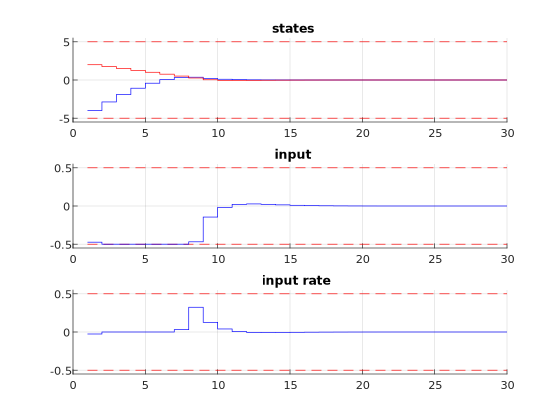
Figure 11.44 Simulation results of the states (top, in blue and red), input (middle, in blue), and input rate change (bottom, in blue) over time.
The constraints are plotted in red dashed lines. The rate constraint is set to 0.5 and is not active at any moment.
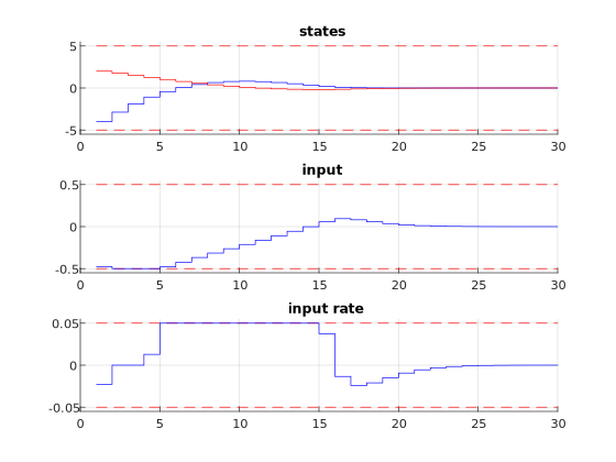
Figure 11.45 Simulation results of the states (top, in blue and red), input (middle, in blue), and input rate change (bottom, in blue) over time.
The constraints are plotted in red dashed lines. The rate constraint is set to 0.05 and is active at some points.