11.6. Low-level interface: Spacecraft Rendezvous (MATLAB & Python)
11.6.1. Introduction
This example uses the concepts described in the subsections HOW TO: Implement an MPC Controller with a Time-Varying Dynamics and How to Implement 1-Norm and Infinity-Norm Cost Functions.
The goal is to design a controller to perform a spacecraft rendezvous operation, where a controlled chaser spacecraft is performing rendezvous with a passive target that is orbiting around Mars. Using a time-varying prediction model allows to perform spacecraft maneuvers in elliptical orbits and allows the controller to be updated when the are changes in the system parameters or control objectives. This example is based on the models described in [HarMac14] and the references therein.
11.6.2. Model
The Yamanaka-Ankersen (Y-A) equations are used to describe the dynamics, where the six states x of the system represent the relative position and velocity of the chaser with respect to the target in the three dimensions. These equations apply in elliptical orbits, but are time-varying in terms of the true anomaly, \(v\), of the target, i.e. the model is given by
and the requirement is that the state at the end of the horizon is at the target. The plant input is modeled as an impulsive change in velocity, such that
You can download a matlab code here with example simulation
here.
The file YA_A_matrix.m computes the time-varying matrices for the prediction horizon given the anomaly \(v\).
11.6.3. Constraints
The three impulsive control inputs can give a maximum change in velocity of 5 meters per second along each axis. In addition, the chaser spacecraft is required to remain within a cone of vision of 20 degrees from the target and must not go behind the target to facilitate the docking maneuver.
11.6.4. Objective
The goal of the controller is to balance the following objectives:
the chaser should be always as close as possible to the target,
use as little fuel as possible to get there.
The second objective is more important, hence it is weighed higher. We consider two types of cost functions: one where all the terms are weighed using standard quadratic penalties; and one where the inputs are penalized using the 1-norm, which better reflects the propellant consumption being directly proportional to delivered thrust and also attempts to minimize the use of the actuators. In order to implement the 1-norm cost we need to add slack variables and additional constraints as described in How to Implement 1-Norm and Infinity-Norm Cost Functions.
The following code shows how to generate an MPC controller for the spacecraft rendezvous problem with a time-varying model and a 1-norm penalty on the actuators.
%% system
nx = 6;         % velocities and acceleration in 3 axes
nu = 3;         % thrusters on 3 axis

%% MPC setup
N = 31;
Q = diag([0.001 0.001 0.001 0 0 0]);
R = diag([15000 15000 15000]);
umin = -5;
umax = 5;
cone_angle = 20*pi/180;
Hx = [1 0 0 0 0 0; ...
      cone_angle 0 1 0 0 0; ...       % Visibility cone
      cone_angle 0 -1 0 0 0];         % Visibility cone
hx = [0; 0; 0];

xs = [-1000; 0; 0; 0; 0; 0];    % target state (1km away)
us = zeros(3,1);

%% FORCESPRO multistage form - 2-norm
% assume variable ordering z(i) = [ui, x_i+1, eu_i] for i=1...N-1

stages = MultistageProblem(N-1);

params(1) = newParam('minusA_times_x0',1,'eq.c'); % RHS of first eq. constr. is a parameter: z1=-A*x0

for i = 1:N-1

        % dimension
        stages(i).dims.n = nx+2*nu; % number of stage variables
        stages(i).dims.r = nx;      % number of equality constraints
        stages(i).dims.l = nu;      % number of lower bounds
        stages(i).dims.u = nu;      % number of upper bounds
        stages(i).dims.p = 3+2*nu;  % number of polytopic constraints

        % cost
        stages(i).cost.H = blkdiag(zeros(nu),Q,zeros(nu));
        stages(i).cost.f = [zeros(nu,1); -Q*xs; ones(nu,1)];

        % lower bounds
        stages(i).ineq.b.lbidx = 1:nu;      % lower bound acts on these indices
        stages(i).ineq.b.lb = umin*ones(nu,1); % lower bound for this stage variable

        % upper bounds
        stages(i).ineq.b.ubidx = 1:nu;      % upper bound acts on these indices
        stages(i).ineq.b.ub = umax*ones(nu,1); % upper bound for this stage variable

        % polytopic bounds
        stages(i).ineq.p.A  = [ zeros(3,nu), Hx, zeros(3,nu); ...
                                R, zeros(nu,nx), -eye(nu); ...
                                -R, zeros(nu,nx), -eye(nu)];
        stages(i).ineq.p.b  = [ hx; R*us; -R*us ];

        % equality constraints
        if( i > 1 )
            stages(i).eq.c = zeros(nx,1);
        end
        params(2*i) = newParam(['D_',num2str(i)],i,'eq.D');
        if( i < N-1 )
            params(2*i+1) = newParam(['C_',num2str(i)],i,'eq.C');
        end

end
nx = 6
nu = 3

N = 31
Q = np.diag([0.001, 0.001, 0.001, 0, 0, 0])
R = np.diag([15000, 15000, 15000])

umin = -5
umax = 5
cone_angle = 20*np.pi/180
Hx = np.array([[1, 0, 0, 0, 0, 0], [cone_angle, 0, 1, 0, 0, 0], [cone_angle, 0, -1, 0, 0, 0]])
hx = np.zeros(3)

xs = np.array([-1000, 0, 0, 0, 0, 0])
us = np.zeros(3)

# assume variable ordering z[i-1] = [ui, x_i+1, eu_i] for i=1...N-1

stages = forcespro.MultistageProblem(N-1)
stages.newParam("minusA_times_xinit", [1], 'eq.c') # 1-indexed

for i in range(N-1):

    # dimensions
    stages.dims[i]['n'] = nx + 2*nu # number of stage variables
    stages.dims[i]['r'] = nx        # number of equality constraints
    stages.dims[i]['l'] = nu        # number of lower bounds
    stages.dims[i]['u'] = nu        # number of upper bounds
    stages.dims[i]['p'] = 3 + 2*nu  # number of polytopic constraints

    # cost
    stages.cost[i]['H'] = block_diag(np.zeros((nu, nu)), Q, np.zeros((nu, nu)))
    stages.cost[i]['f'] = np.concatenate([np.zeros(nu), -Q @ xs, np.ones(nu)])

    # lower bounds
    stages.ineq[i]['b']['lbidx'] = range(1, nu + 1)   # 1-indexed, lower bound acts on these indices
    stages.ineq[i]['b']['lb'] = umin*np.ones(nu) # lower bound for this stage variable

    # upper bounds
    stages.ineq[i]['b']['ubidx'] = range(1, nu + 1)   # 1-indexed, upper bound acts on these indices
    stages.ineq[i]['b']['ub'] = umax*np.ones(nu) # upper bound for this stage variable

    # polytopic bounds
    stages.ineq[i]['p']['A'] = np.block([[np.zeros((3, nu)), Hx, np.zeros((3, nu))],
                                         [R, np.zeros((nu, nx)), -np.eye(nu)],
                                         [-R, np.zeros((nu, nx)), -np.eye(nu)]])
    stages.ineq[i]['p']['b'] = np.concatenate([hx, R @ us, -R @ us])

    # equality constraints
    if i > 0:
        stages.eq[i]['c'] = np.zeros(nx)

    stages.newParam(f"D_{i+1}", [i+1], 'eq.D') # 1-indexed

    if i < N-2:
        stages.newParam(f"C_{i+1}", [i+1], 'eq.C') # 1-indexed
11.6.5. Spacecraft Rendezvous Maneuvers with and without 1-Norm Cost
The simulation describes a rendezvous maneuver were the chaser starts 15km away from the target spacecraft and the goal is to approach the target to within 1000 meter distance, while respecting the constraints, to start the docking maneuver. The target is modeled as being in a Keplerian orbit around Mars with an orbital radius of 3,600,000 meters. The controller sampling time is 200s but the target and chaser dynamics are simulated in intervals of 1s for illustration purposes. The plots in Figure 11.25 illustrates the behavior of the controlled spacecraft with standard quadratic cost, while the plots in Figure 11.26 shows the behavior of the controller when the quadratic cost on the actuators is swapped with a 1-norm penalty. Notice the sparsity in the actuation commands - the thrusters are only engaged when necessary to keep the spacecraft within the cone of visibility of the target.
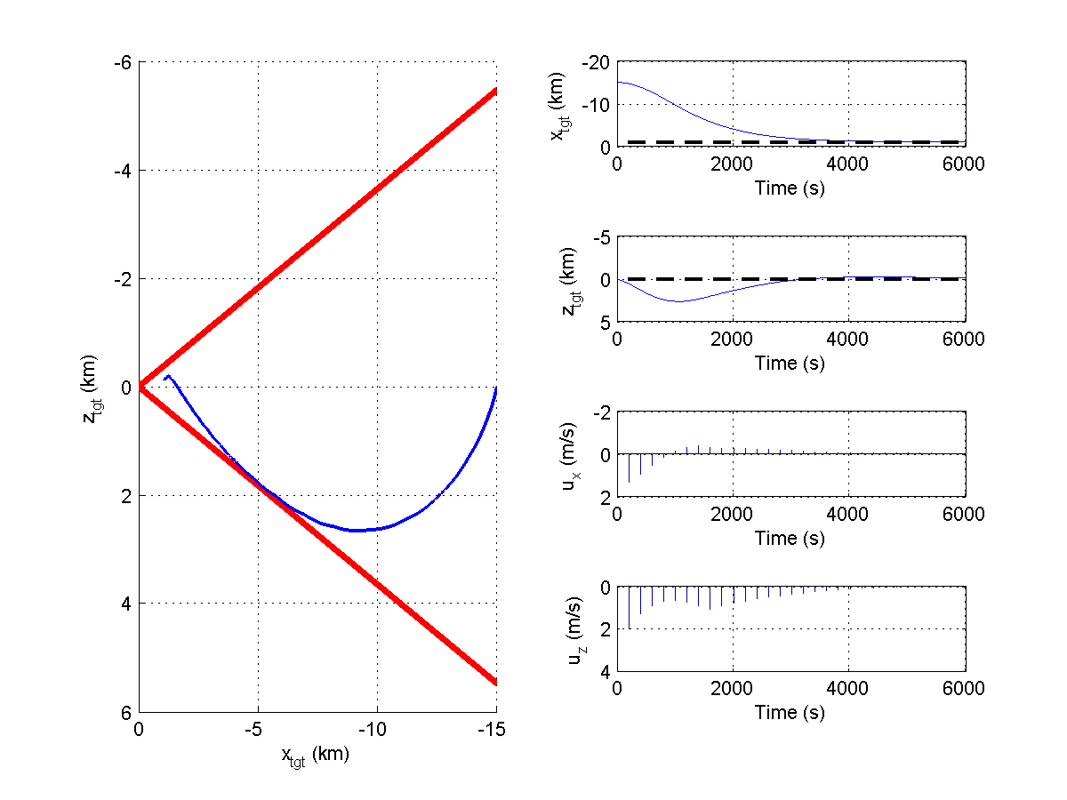
Figure 11.25 Behavior with quadratic cost.
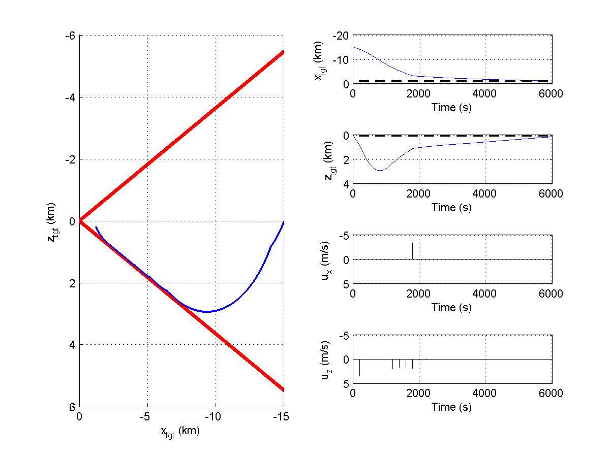
Figure 11.26 Behavior with cost given by 1-norm.
Hartley, E. N.; Maciejowski, J. M.: Field programmable gate array based predictive control system for spacecraft rendezvous in elliptical orbits. In Optimal Control Applications and Methods, Mar 2014