11.4. Low-level interface: Active Suspension Control

11.4.1. Introduction

The concept of using future information, as described in the section How to Incorporate Preview Information in the MPC Problem can be applied to more advanced systems. In this example a driving vehicle is considered, equipped with sensors that measure the unevenness of the road ahead as shown in the picture below.

Figure 11.11 Figure borrowed from [GörSch]

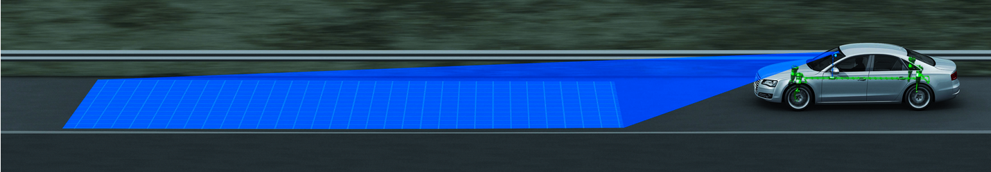
The preview information can be used to improve the riding comfort, i. e. minimize the heave, pitch and roll accelerations, by actively controlling the suspension of the vehicle. This example is based on the reduced car model described in [GörSch]

The states \(x\) of the system are ‘heave displacement’ \(z_b\) [m], ‘pitch angle’ \(\varphi\) [rads], ‘roll angle’ \(\theta\) [rads], ‘heave velocity’ \(\dot{z}_b\) [m/s], ‘pitch rate’ \(\dot{\varphi}\) [rads/s] and ‘roll rate’ \(\dot{\varphi}\) [rads/s]. The input \(u\) [m] to the system are the ‘active spring displacements’. The output \(y\) is given by the ‘heave acceleration’ \(\ddot{z}_b\) \(\text{[m/s}^2\text{]}\), the ‘pitch acceleration’ \(\ddot{\varphi}\) \(\text{[m/s}^2\text{]}\) and the ‘roll acceleration’ \(\ddot{\theta}\) \(\text{[m/s}^2\text{]}\). In the reduced model, the input contains not only the active spring displacements but also the measurements of the height profile of the upcoming road \(w\) and its first derivative \(\dot{w}\).

\begin{align*} x &:= \begin{pmatrix} \text{heave displacement [m]} \\ \text{pitch angle [rads]} \\ \text{roll angle [rads]} \\ \text{heave velocity [m/s]} \\ \text{pitch rate [rads/s]} \\ \text{roll rate [rads/s]} \end{pmatrix} \\ u &:= \begin{pmatrix} \text{active spring displacements [m]} \end{pmatrix} \\ y &:= \begin{pmatrix} \text{heave acceleration [m/s$^2$]} \\ \text{pitch acceleration [rads/s$^2$]} \\ \text{roll acceleration [rads/s$^2$]} \end{pmatrix} \end{align*}

There are constraints on the actuators, i. e. minimal and maximal adjustment track, \(\underline{u} = - 0.04 [m]\) and \(\overline{u} = 0.04 [m]\). This results in the following state space system:

\begin{align*} \dot{x}(t)&= Ax(t)+B_u u(t)+ B_w \begin{pmatrix} w(t) \\ \dot{w}(t) \end{pmatrix} \\ y(t) &= Cx(t) + Du(t) \end{align*}

In the following it is shown how the FORCESPRO MATLAB Interface can be used to design a controller using preview information, substantially increasing the riding comfort compared to a vehicle with a passive suspension. The discrete vehicle model is sampled at 0.025 [s] and it is assumed that road preview information for 0.5 [s] (20 steps) is available to the controller.

11.4.2. Disturbance Model: Speed Bump

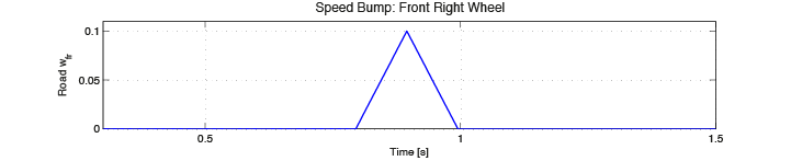
The vehicle is assumed to be driving at a constant speed of 5 [m/s] over a speed bump of length 1 [m] with a height of 0.1 [m]. The disturbance in time domain is depicted on the right side. The road bump only hits the front right wheel, while the front left wheel is not affected. The same bump will hit the rear right wheel 1.12 [s] after it hits the front wheel.

11.4.3. Implementation of Preview Information

This is a linear MPC problem with lower and upper bounds on inputs and a terminal cost term:

\begin{align*} \text{minimize}\quad & x_N^TPx_N + \sum_{i=0}^{N-1}x_i^TQx_i + u_i^TRu_i \\ \text{subject to}\quad & x_0=x \\ & x_{i+1}=Ax_i + Bu_i + B_ww_i + B_w \dot{w}_i \\ & \underline{u}\leq u_i \leq \overline{u} \end{align*}

At each sampling instant the initial state \(x\) and the preview information \(w_i\) and \(\dot{w}_i\) change, and the first input \(u_0\) is typically applied to the system after an optimal solution has been obtained.

% Parameters: First Equation RHS
parameter(1) = newParam('minusA_times_x0_minusBw_times_w_pre',1,'eq.c');
% Parameters: Preview Information
parameter(2) = newParam('pre2_w',2,'eq.c');
...
parameter(n) = newParam('pren_w',n,'eq.c');
...
parameter(N) = newParam('preN_w',N,'eq.c');

As described in the section How to Incorporate Preview Information in the MPC Problem, the parametric additive terms g, which corresponds to the term \(B_w wi+B_w \dot{w}_i\), has to be defined. At each stage of the multistage problem, the ‘g’ term (containing the preview information) in the equality constraint is different, therefore we have to define a parameter for each stage. In the definition of the parameters, ‘pren_w’ represents the name of the term \(B_w w_n+B_w \dot{w}_n\) at stage \(n\) of the multistage problem. During runtime, the preview information is mapped to these parameters.

\(N\) is the length of the prediction horizon which is set to be equal to the preview horizon. The MATLAB code below, generates the function VEHICLE_MPC_withPreview that takes -\(Ax\) and the additive term g as a calling argument and returns \(u_0\), which can then be applied to the system:

%% MPC with Preview
% FORCESPRO multistage form
% assume variable ordering zi = [u{i-1}; x{i}] for i=1...N

% Parameters: First Eq. RHS
parameter(1) = newParam('minusA_times_x0_minusBw_times_w_pre’,1,'eq.c’);

stages = MultistageProblem(N);
for i = 1:N

   % dimension
   stages(i).dims.n = nx+nu; % number of stage variables
   stages(i).dims.r = nx; % number of equality constraints
   stages(i).dims.l = nu; % number of lower bounds
   stages(i).dims.u = nu; % number of upper bounds

   % cost
   if( i == N )
          stages(i).cost.H = blkdiag(R,P);
   else
          stages(i).cost.H = blkdiag(R,Q);
   end
   stages(i).cost.f = zeros(nx+nu,1);

   % lower bounds
   stages(i).ineq.b.lbidx = 1:nu; % lower bound acts on these indices
   stages(i).ineq.b.lb = umin*ones(4,1); % lower bound for the input signal

   % upper bounds
   stages(i).ineq.b.ubidx = 1:nu; % upper bound acts on these indices
   stages(i).ineq.b.ub = umax*ones(4,1); % upper bound for the input signal

   % equality constraints
   if( i < N )
          stages(i).eq.C = [zeros(nx,nu), Ad];
   end
   stages(i).eq.D = [Bdu, -eye(nx)];

   % Parameters for Preview
   if (i > 1)
       parameter(i)  = newParam(['pre',num2str(i),'_w'],i,'eq.c');
   end

end

% define outputs of the solver
outputs(1) = newOutput('u0',1,1:nu);

% solver settings
codeoptions = getOptions('VEHICLE_MPC_withPreview');

% generate code
generateCode(stages,parameter,codeoptions,outputs);

You can download the MATLAB code of this example to try it out for yourself by clicking here.

11.4.4. Comparison of Passive Vehicle and Active Suspension Control Using Preview Information

In Figure 11.12, Figure 11.13 and Figure 11.14, the accelerations in the direction heave, pitch and roll respectively are depicted. The blue graphs represent the controlled outputs while the red ones show the uncontrolled accelerations. One can see that the vertical dynamics of the vehicle are reduced substantially. There are smaller maximal accelerations and also less time is required to regulate the accelerations back to zero.

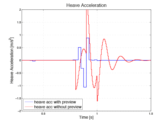
Figure 11.12 Acceleration in heave direction

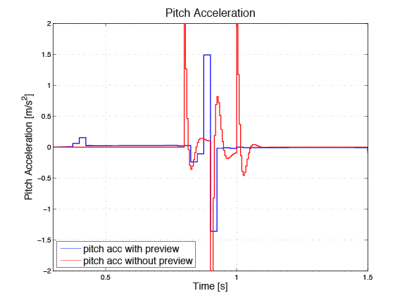
Figure 11.13 Acceleration in pitch direction

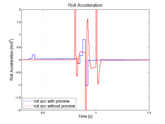
Figure 11.14 Acceleration in roll direction

Applying Model Predictive Control with Preview using FORCESPRO the riding comfort is improved significantly with minimum effort for designing the controller and generating code which can be deployed on any embedded automotive control unit.

The four graphs in Figure 11.15, Figure 11.16, Figure 11.17 and Figure 11.18 below show the input signal on each of the four actuators. One can see that model predictive controller starts lifting the front right part of the vehicle body as soon as the bump is in sight of the preview sensor, i. e. at time \(t = 0.3\) [s]. This is \(0.5\) seconds, the length of the preview horizon, before the front right wheel hits the bump at time \(t = 0.8\) [s]. This causes a better absorption of the shock and therefore reduced accelerations. The input constraints are also satisfied and \(u\) never exceeds the admitted range.

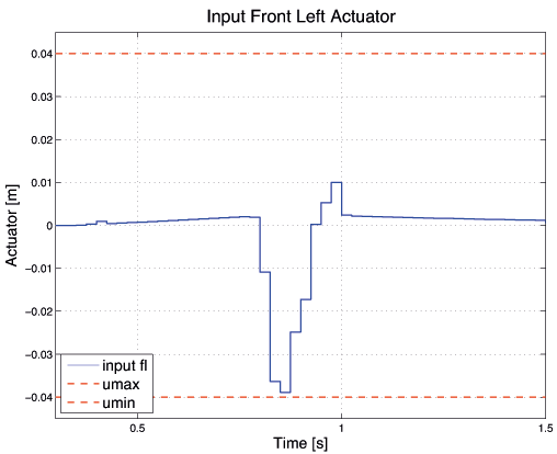
Figure 11.15 Input front left actuator

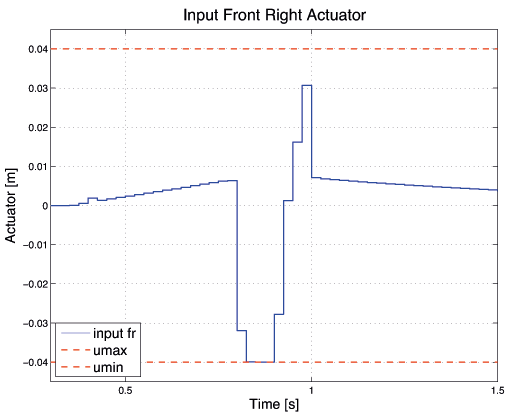
Figure 11.16 Input front right actuator

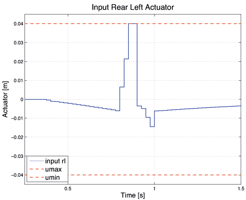
Figure 11.17 Input rear left actuator

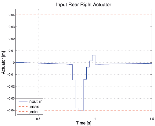
Figure 11.18 Input rear right actuator

[GörSch] (1,2)

Göhrle, C.; Schindler, A.; Wagner, A.; Sawodny, O.: Design and Vehicle Implementation of Preview Active Suspension Controllers. IEEE Transactions on Control Systems Technology, pp.1135–1142, vol. 22, no. 3, May 2014