11.18. Mixed-integer nonlinear solver: F8 Crusader aircraft
In this example we illustrate the simplicity of the high-level user interface on a mixed-integer nonlinear program. In particular, we use an F8 Crusader aircraft model described by a set of ordinary differential equations (ODEs):
The model is taken from [GarJor77] and consists of three differential states: \(x_0\) the angle of attack in radians, \(x_1\) the pitch angle in radians and \(x_2\) the pitch angle rate in radians per second. There is one control input \(w\), the tail deflection angle in radians. The input is the discrete component of the model, since it can take values within the discrete set \(\{-0.05236, 0.05236\}\). This makes the solution process more complicated in comparison to a nonlinear program, as the different combinations of inputs have to be checked over the control horizon.
The trajectory of the aircraft is to be computed by solving a mixed-integer nonlinear program (MINLP). First, we define the stage variable \(z\) by stacking the input and differential state variables:
You can download the MATLAB code of this example to try it out for yourself by
clicking here.
11.18.1. Defining the problem data
11.18.1.1. Objective
Our goal is to minimize the distance of the final state to the origin, which can be translated in the following cost function on the final stage variable:
The terminal cost function is coded in MATLAB as the following function:
model.objectiveN = @(z) 150 * z(2)^2 + 5 * z(3)^2 + 5 * z(4)^2;
Moreover, control inputs are penalized at every stage via the following stage cost function:
model.objective = @(z) 0.0001 * z(1)^2;
11.18.1.2. Equality constraints
In this example, the only equality constraints are related to the dynamics. They are provided to FORCESPRO in continuous form. The discretization is then computed internally by the FORCESPRO integrators.
In the code snippet below, it is important to notice that the control input \(w\) is replaced with \(u\) such that
If \(w\) has values within \(\{-0.05236, 0.05236\}\), then \(u\) lies within the binary set \(\{0, 1\}\).
wa = 0.05236;
  wa2 = wa^2;
  wa3 = wa^3;
  continuous_dynamics = @(x, u) [ -0.877 * x(1) + x(3) - 0.088 * x(1) * x(3) + 0.47 * x(1) * x(1) - 0.019 * x(2) * x(2) - x(1) * x(1) * x(3)...
                                  + 3.846 * x(1) * x(1) * x(1) - 0.215 * wa * (2 * u(1) - 1) + 0.28 * x(1) * x(1) * wa * (2 * u(1) - 1) + 0.47 * x(1) * wa2 * (2 * u(1) - 1) * (2 * u(1) - 1)...
                                  + 0.63 * wa3 * (2 * u(1) - 1) * (2 * u(1) - 1) * ( 2 * u(1) - 1);
                                  x(3);
                                  -4.208 * x(1) - 0.396 * x(3) - 0.47 * x(1) * x(1) - 3.564 * x(1) * x(1) * x(1) - 20.967 * wa * (2 * u(1) - 1) + 6.265 * x(1) * x(1) * wa * (2 * u(1) -1 )...
                                  + 46.0 * x(1) * wa2 * (2 * u(1) - 1) * (2 * u(1) - 1) + 61.4 * wa3 * (2 * u(1) - 1) * (2 * u(1) - 1) * (2 * u(1) - 1)];
  model.continuous_dynamics = continuous_dynamics;
  model.E = [zeros(params.dimX, params.dimU), eye(params.dimX)];
11.18.1.3. Inequality constraints
The maneuver is subjected to a set of constraints, involving only the simple bounds:
11.18.1.4. Initial and final conditions
The goal of the maneuver is to steer the aircraft from an initial condition with nose pointing upwards
to the origin.
11.18.2. Defining the MPC problem
With the above defined MATLAB functions for objective and equality constraints, we can completely define the MINLP formulation in the next code snippet. For this example, the number of stages has been set to \(N = 100\).
In the code snippet below, it is important to notice that the lower and upper bounds are declared as parametric before generating the solver. This needs to be done for generating mixed-integer NLP solvers. Lower and upper bounds are meant to be provided at run-time.
Nstages = 100;

params.dimU = 1;
params.dimX = 3;
params.dimZ = params.dimU + params.dimX;

%% Model with stage variable (u', x')'
model.N = Nstages;
model.nvar = params.dimZ;
model.neq = params.dimX;

%% Boundary conditions
model.xinitidx = params.dimU+1:model.nvar;

%% Bounds
model.lb = [];
model.ub = [];
model.lbidx{1} = 1 : params.dimU;
model.ubidx{1} = 1 : params.dimU;
for i = 2 : model.N
    model.lbidx{i} = 1 : model.nvar;
    model.ubidx{i} = 1 : model.nvar;
end

%% Dynamics
wa = 0.05236;
wa2 = wa^2;
wa3 = wa^3;
continuous_dynamics = @(x, u) [ -0.877 * x(1) + x(3) - 0.088 * x(1) * x(3) + 0.47 * x(1) * x(1) - 0.019 * x(2) * x(2) - x(1) * x(1) * x(3)...
                                + 3.846 * x(1) * x(1) * x(1) - 0.215 * wa * (2 * u(1) - 1) + 0.28 * x(1) * x(1) * wa * (2 * u(1) - 1) + 0.47 * x(1) * wa2 * (2 * u(1) - 1) * (2 * u(1) - 1)...
                                + 0.63 * wa3 * (2 * u(1) - 1) * (2 * u(1) - 1) * ( 2 * u(1) - 1);
                                x(3);
                                -4.208 * x(1) - 0.396 * x(3) - 0.47 * x(1) * x(1) - 3.564 * x(1) * x(1) * x(1) - 20.967 * wa * (2 * u(1) - 1) + 6.265 * x(1) * x(1) * wa * (2 * u(1) -1 )...
                                + 46.0 * x(1) * wa2 * (2 * u(1) - 1) * (2 * u(1) - 1) + 61.4 * wa3 * (2 * u(1) - 1) * (2 * u(1) - 1) * (2 * u(1) - 1)];
model.continuous_dynamics = continuous_dynamics;
model.E = [zeros(params.dimX, params.dimU), eye(params.dimX)];

%% Objective
model.objective =  @(z) 0.0001 * z(params.dimU)^2;
model.objectiveN = @(z) 150 * z(params.dimU+1)^2 + 5 * z(params.dimU+2)^2 + 5 * z(params.dimU+3)^2;

%% Integer indices
for s = 1:model.N
    model.intidx{s} = 1;
end

%% Define outputs
outputs(1) = newOutput('TailAngle', 1:model.N, 1);
outputs(2) = newOutput('AngleAttack', 1:model.N, 2);
outputs(3) = newOutput('PitchAngle', 1:model.N, 3);
outputs(4) = newOutput('PitchAngleRate', 1:model.N, 4);
11.18.3. Generating an MINLP solver
We have now populated model with the necessary fields to generate a mixed-integer solver
for our problem. Now we set some options for our solver and then use the
function FORCES_NLP to generate a solver for the problem defined by
model with the initial state and the lower and upper bounds as a parameters:
%% Set code-generation options
codeoptions = getOptions('F8aircraft_solver');
codeoptions.printlevel = 0;
codeoptions.maxit = 2000;
codeoptions.timing = 0;
codeoptions.nlp.integrator.type = 'IRK2';
codeoptions.nlp.integrator.Ts = 0.05;
codeoptions.nlp.integrator.nodes = 20;
% Specify maximum number of threads to parallelize minlp search
codeoptions.minlp.max_num_threads = 8;

%% Generate MINLP solver
FORCES_NLP(model, codeoptions, outputs);
In the code snippet above, we have set some integrator options, since the continuous-time dynamics has been provided in the model. The branch-and-bound search can be run on several threads in parallel by setting the run-time parameter numThreadsBnB equal to the number of threads to be used. The default value is 1. Moreover, the maximum number of threads for the branch-and-bound search can be set via the option max_num_threads. By default, max_num_threads = 4.
11.18.4. Calling the generated MINLP solver
Once all parameters have been populated, the MEX interface of the solver can be used to invoke it:
%% Set run-time parameters
model.nu = params.dimU;
model.nx = params.dimX;
problem.(sprintf('lb%03d', 1)) = 0;
problem.(sprintf('ub%03d', 1)) = 1;
for s = 2:Nstages-1
    problem.(sprintf('lb%03d', s)) = [0, -1e1 * ones(1, model.nx)]';
    problem.(sprintf('ub%03d', s)) = [1, 1e1 * ones(1, model.nx)]';
end
problem.(sprintf('lb%03d', Nstages)) = [0, -1e1 * ones(1, model.nx)]';
problem.(sprintf('ub%03d', Nstages)) = [1, 1e1 * ones(1, model.nx)]';

problem.x0 = repmat([0; zeros(model.nx, 1)], Nstages, 1);
problem.xinit = zeros(model.nx, 1);
problem.xinit(1) = 0.4655;

%% Call MINLP solver
[sol, exitflag, info] = F8aircraft_solver(problem);
11.18.5. Providing an initial guess at run-time
In order to provide an guess for the incumbent, the following code-generation options need to be enabled:
codeoptions.minlp.int_guess = 1;
codeoptions.minlp.round_root = 0; % Default value is 1
codeoptions.minlp.int_guess_stage_vars = [1]; % An integer guess is provided for variable 1 at every stage
Then the incumbent guess can be set at run-time via
for s = 1:Nstages
  problem.(sprintf('int_guess%03d', s)) = [0];
end
for s = 1:2
  problem.(sprintf('int_guess%03d', s)) = [1];
end
problem.(sprintf('int_guess%03d', 39)) = [1];
for s = 41:42
  problem.(sprintf('int_guess%03d', s)) = [1];
end
for s = 85:90
  problem.(sprintf('int_guess%03d', s)) = [1];
end
11.18.6. Changing the parallelization strategy at run-time
When running the MINLP solver on several threads with numThreadsBnB >= 1, the parallelization strategy can be changed via
problem.parallelStrategy = 0; % 0 (one shared priority queue, default), 1 (one priority queue per thread)
11.18.7. Results
The control objective is to drive the angle of attack as close as possible to zero within a five seconds time frame. The control input is the tail deflection angle, which can take values with the set \(\{-0.05236, 0.05236\}\) and the initial state is \((0.4655, 0, 0)^{T}\), where the first component is the angle of attack, the second component is the pitch angle and the third component is the pitch angle rate.
The angle of attack computed by FORCESPRO MINLP solver running on one thread is shown in Figure Figure 11.58 and the input sequence is in Figure Figure 11.59. One can notice the bang-bang behavior of the solution. When running on three threads the FORCESPRO MINLP solver provides a solution with lower final primal objective. Results are shown on Figures Figure 11.60 and Figure 11.61.
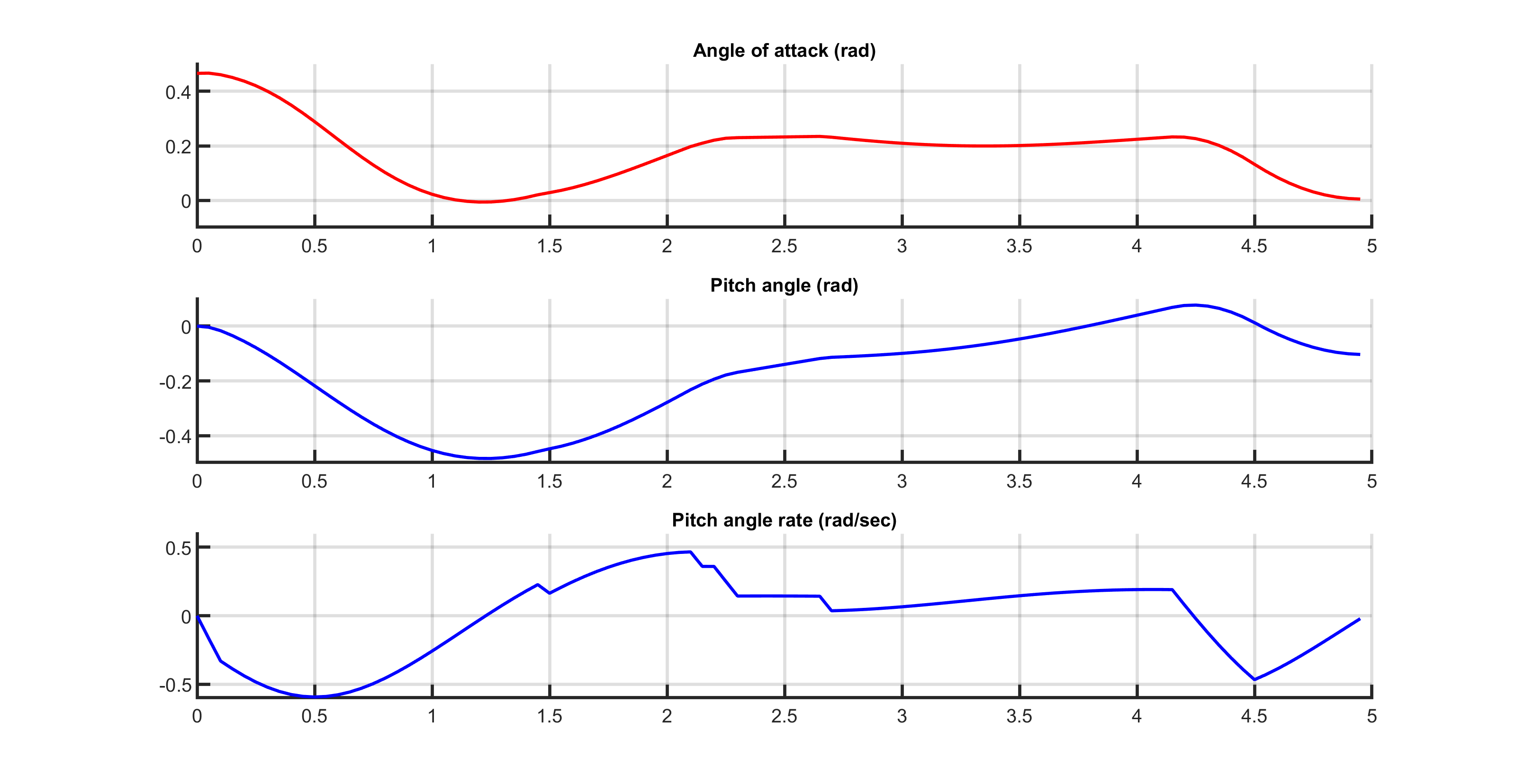
Figure 11.58 Aircraft’s angle of attack over time computed with one thread.
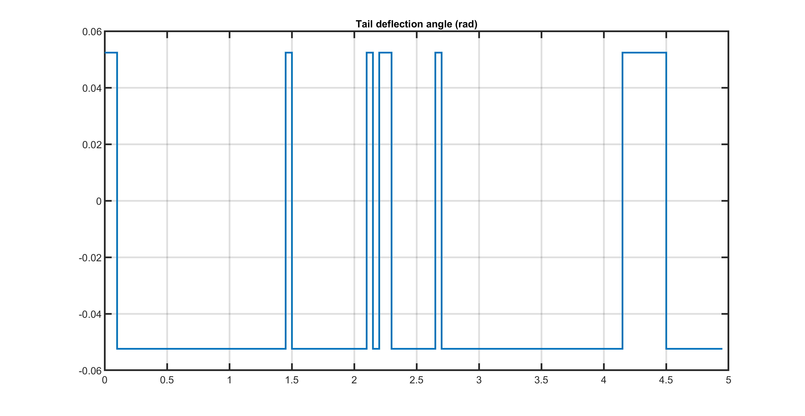
Figure 11.59 Aircraft’s tail deflection angle over time with one thread.
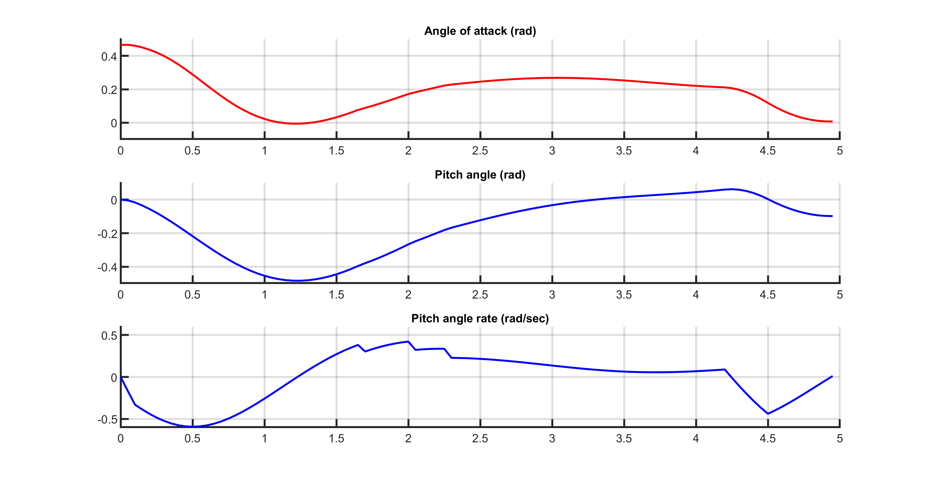
Figure 11.60 Aircraft’s angle of attack over time computed with three threads.
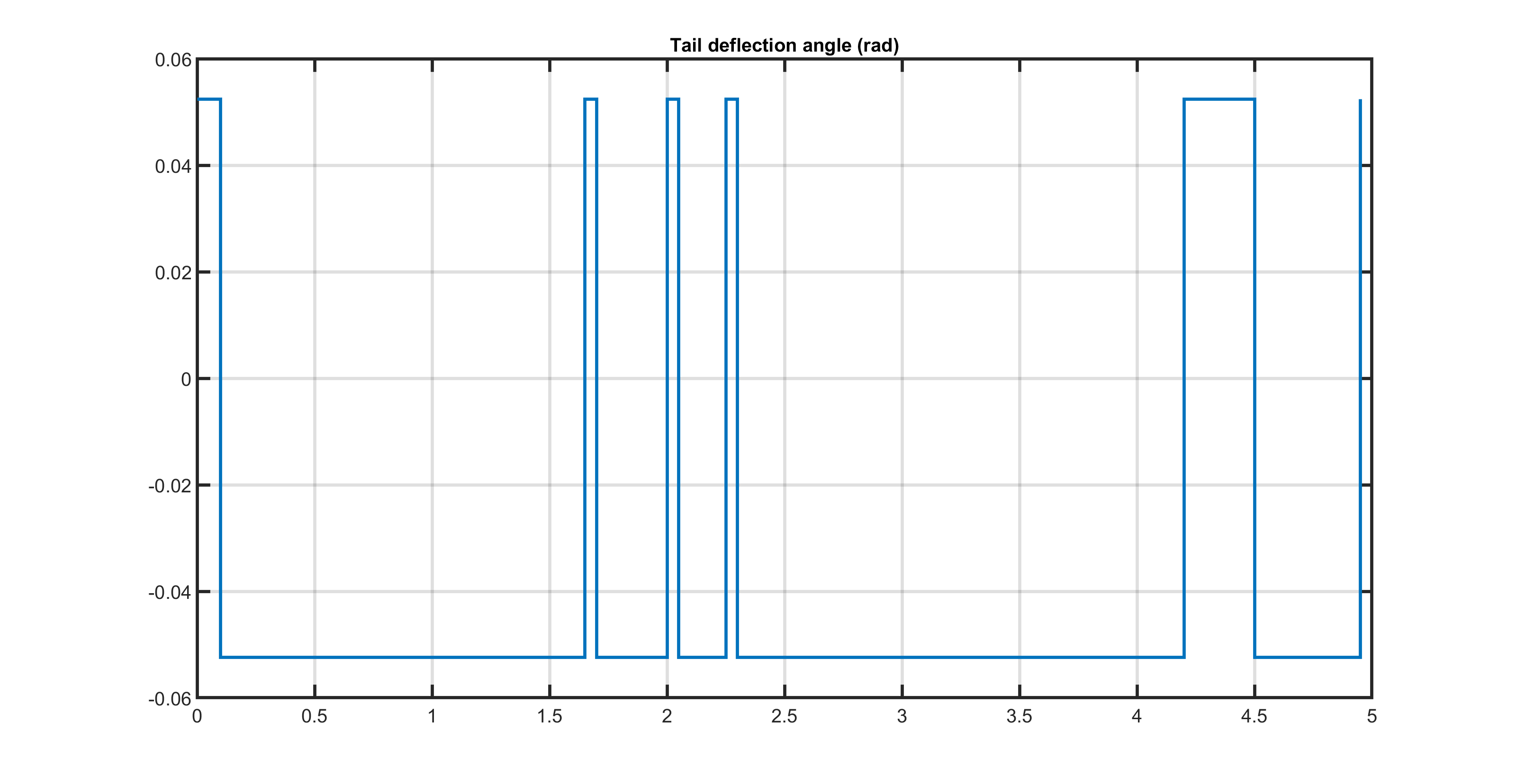
Figure 11.61 Aircraft’s tail deflection angle over time with three threads.
Garrard, W.L.; Jordan, J.M..: Design of Nonlinear Automatic Control Systems. In: Automatica 1977, vol. 13, 497-505.