10.4.1. Getting Started - Basic MPC Regulation State Feedback Example
This example will show how to get started with the Simulink® interface(s) of FORCESPRO by designing an MPC regulator for the system below.
You can download the MATLAB code of this example to try it out for yourself by
clicking here.
This example can be used to show the workflow both for the S-Function interface and the Coder interface.
10.4.1.1. Generating the FORCESPRO solver
The state-space model of the system has been obtained by discretizing the continuous model with a sampling time of \(0.1\) seconds, and can be described by
In addition to the task of steering the two states to zero, there are constraints on the single actuator \(u\) and on the second state \(x_2\). We require that the actuator \(u\) does not exceed \([−5,5]\) and the state \(x_2 \geq 0\) for all time steps.
After downloading the files we can start with the design of the controller. First open and run the script examples/Matlab/SimulinkInterface/generateMyFirstController.m. This script will define the underlying MPC problem and generate the FORCESPRO solver.
First we define the MPC problem parameters, i.e. the state transition matrix \(A\) and the input matrix \(B\). The output matrix \(C\) and the feed-forward matrix \(D\) are not needed for solver generation, but are used in the Simulink® workspace to define the state-space parameters of the dynamical system block. Notice that we use the identity output matrix, since we want to regulate both states and not just the output of the system.
% MPC parameter setup

% system
A = [0.7115 -0.4345; 0.4345 0.8853];
B = [0.2173; 0.0573];
[nx,nu] = size(B);
C = eye(nx);
D = zeros(nx,1);

% horizon length
N = 10;

% weights in the objective
R = eye(nu);
Q = 10*eye(nx);

% bounds
umin = -5;     umax = 5;
xmin = [-inf, 0]; xmax = [+inf, +inf];
We choose a prediction horizon of \(10\) steps, i.e. the controller looks \(1\) second into the future. We define the relative weights in the objective function by prioritizing the importance of regulating the states \(10\) times higher than reducing the use of the actuator. You are encouraged to change these weights and observe the effect on the control behavior.
We also input the details of the constraints described above. The second state must remain positive, whereas the first state is left unconstrained. We also have a constraint on the actuator, with the lower bound \(−5\) and the upper bound \(5\).
Next, we define the model struct describing the multistage MPC problem formulation. This includes the model dynamics (i.e. equality constraints), as well as the bounds on state and control variables in the form of inequality constraints.
% FORCESPRO multistage form
% assume variable ordering zi = [ui; xi] for i=1...N

% dimensions
model.N     = N;        % horizon length
model.nvar  = nx+nu;    % number of variables
model.neq   = nx;       % number of equality constraints

% objective
model.objective = @(z) z(1)*R*z(1) + [z(2);z(3)]'*Q*[z(2);z(3)];

% equalities
model.eq = @(z) [ A(1,:)*[z(2);z(3)] + B(1)*z(1);
                        A(2,:)*[z(2);z(3)] + B(2)*z(1)];

model.E = [zeros(2,1), eye(2)];

% inequalities
model.lb = [umin, xmin];
model.ub = [umax, xmax];

% initial state
model.xinitidx = 2:3;
Finally, we generate the FORCESPRO solver called myFirstController. Since we will incorporate the solver in the Simulink® model, we confine the output to the first element of the solution vector at stage 1, corresponding to the actuator control action of interest.
% Generate FORCESPRO solver

% get options
codeoptions = getOptions('myFirstController');
codeoptions.printlevel = 2;
codeoptions.BuildSimulinkBlock = 1;

% generate code
output1 = newOutput('u0', 1, 1);
FORCES_NLP(model, codeoptions, output1);
This will send a request to the server which will generate a custom controller for your problem.
The code is downloaded to your machine and the appropriate Simulink® block and Simulink® S-function can be found inside the interface folder.
We also provide additional initialization parameters needed for the Simulink® model.
% Model Initialization (needed for Simulink® only)

% initial conditions
x_init = [0; 6];

% initial guess
x0 = zeros(model.N*model.nvar,1);
We can now open the Simulink® model myFirstController_sim.slx (by copying the myFirstController_sim_template.slx file) and incorporate the generated solver into the Simulink® diagram.
10.4.1.2. Workflow for S-Function interface
In this example we will use the compact FORCESPRO Simulink® block myFirstControllercompact_lib.mdl (see Real-time control with the Simulink® block for more details). We open myFirstControllercompact_lib.mdl and copy the FORCESPRO Simulink® block to the myFirstController_sim.slx Simulink® model.
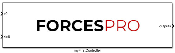
Figure 10.1 Preview of the generated FORCESPRO Simulink® block.
The port labels are self-explanatory. All we have to do is wire the ports of the FORCESPRO block to other blocks in your Simulink® diagram and run the simulation.
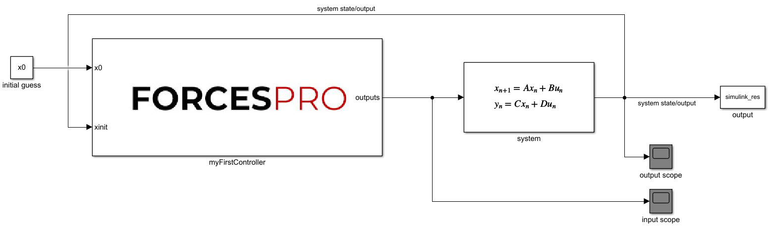
Figure 10.2 Simulink® diagram of the model with inclusion of the FORCESPRO Simulink® block.
10.4.1.3. Workflow for Coder interface
We change the Solver of the Simulink® model to Fixed-Step as the Coder interface does not support Variable-Step.
% the coder interface only supports Fixed-Step Simulations
set_param('myFirstController_sim', 'Solver', 'FixedStep');
In this example we will use the compact FORCESPRO Simulink® block. To add the Simulink® block to the myFirstController_sim.slx Simulink® model we run the myFirstController_createCoderMatlabFunction.m from the interface folder.
% add the interface folder to the path
addpath(fullfile('myFirstController', 'interface'));

% for the coder case run myFirstController_createCoderMatlabFunction in
% myFirstController/interface to create a FORCESPRO Simulink® block to
% the Simulink® model:
%     * The first parameter is the target Simulink® model
%     * The second parameter is the name of the created Simulink® model
%     * The third parameter selects whether to use the standard or the
%       compact version
%     * The fourth parameter must be set to true if the Simulink® model
%       already exists (by default the script always tries to create a
%       new Simulink® model)
myFirstController_createCoderMatlabFunction('myFirstController_sim', 'myFirstController', true, true);

% (optionally) remove the interface folder from the path again
rmpath(fullfile('myFirstController', 'interface'));
10.4.1.4. Simulation and checking of results
From the left plot we can see that the actuator remains in the allowed range. The right plot shows how the second state \(x_2\) is always non-negative (purple graph in the right plot) and both states are regulated to zero.
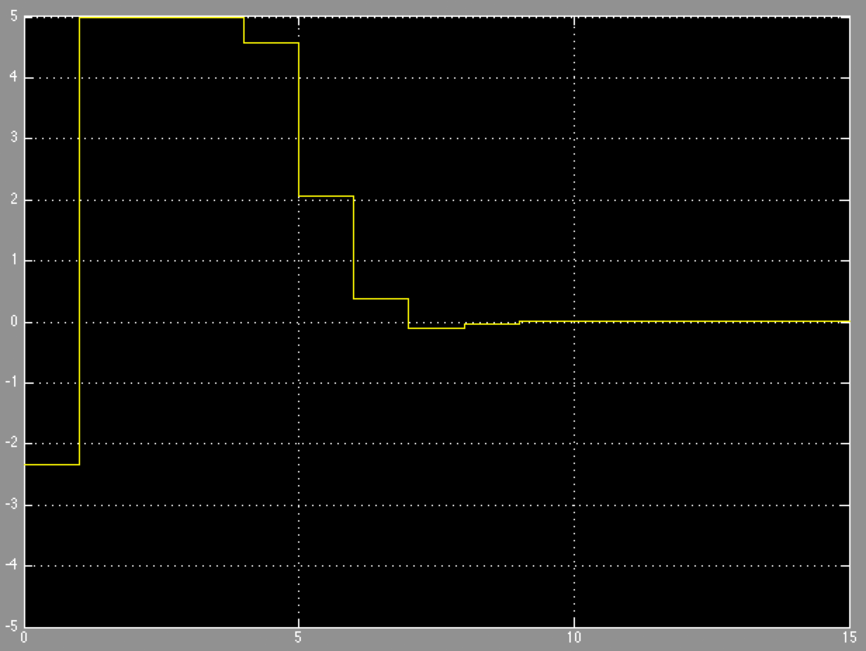
Figure 10.3 Actuator control signal.
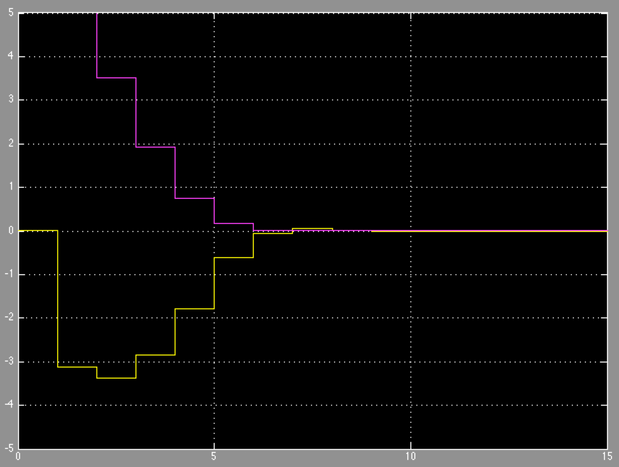
Figure 10.4 State evolution of the system.