11.11. High-level interface: Path tracking example (MATLAB)

In this example we illustrate the simplicity of the SQP_NLP API on a path-tracking problem. We also illustrate the full workflow for the SQP Fast solver which must be tuned to the specific application. See Using the SQP Fast solver for specifics on the workflow for the SQP Fast solver. In every simulation step, the predicted trajectory of the car is optimized to follow a set of path points, either an ellipse or an artificial racetrack. The example visualizes how the predicted trajectory changes while the car moves along the path.

We use a kinematic bicycle model described by a set of ordinary differential equations (ODEs):

\[\begin{split}\dot{x} & = v \cos(\theta + \beta) \\ \dot{y} & = v \sin(\theta + \beta) \\ \dot{v} & = \frac{F}{m} \\ \dot{\theta} & = \frac{v}{l_r} \sin(\beta) \\ \dot{\delta} &= \phi\end{split}\]

with:

\[\beta = \arctan\left( \frac{l_r}{l_r + l_f} \tan( \delta)\right)\]

The model consists of five differential states: \(x\) and \(y\) are the Cartesian coordinates of the car, and \(v\) is the linear velocity. The angles \(\theta\) and \(\delta\) denote the heading angle of the car and its steering angle, respectively. Next, there are two control inputs to the model: the longitudinal acceleration force \(F\) and the steering rate \(\phi\). The angle \(\beta\) describes the direction of movement of the car’s center of gravity relative to the heading angle \(\theta\). The remaining three constant parameters of the system are the car mass \(m=1\,\mathrm{kg}\), and the lengths \(l_r=0.5\,\mathrm{m}\) and \(l_f=0.5\,\mathrm{m}\) specifying the distance from the car’s center of gravity to the rear wheels and the front wheels, respectively.

The trajectory of the vehicle will be defined as an NLP. First, we define stage variable \(z\) by stacking the input and differential state variables:

\[z = [F,\phi,x,y,v,\theta,\delta]^\top\]

You can download the code of this example using SQP General here (MATLAB) and SQP Fast here (MATLAB)

11.11.1. Defining the MPC Problem

11.11.1.1. Objective

In this example the cost function is the same for all stages except for the last stage N. The objective of this example is to follow a set of path points. At runtime, a target position \(p_i\) for each stage \(i\) is provided. Each point consists of a x- and a y-coordinate:

\[p_i = [p_{i,x}, p_{i,y}]^\top\]

The goal is to minimize the distance of the car to these target points. The distance is penalized with quadratic costs. Plus, some small quadratic costs are added to the inputs \(F\) and \(s\), i.e.:

\[f(z,p_i) = 200 (z_3 - p_{i,x})^2 + 200 (z_4 - p_{i,y})^2 + 0.2 z_1^2 + 10 1 z_2^2\]

Since all cost terms are quadratic and summed up, we can formulate the objective as a least squares problem:

\[\begin{split}f(z,p_i) & = \frac{1}{2} || r(z,p_i) ||_2^2 \\ r(z,p_i) & = [ \sqrt{200} (z_3 - p_{i,x}), \sqrt{200} (z_4 - p_{i,y}), \sqrt{0.2} z_1, \sqrt{10.0} z_2 ]^\top\end{split}\]

The stage cost function is coded in MATLAB as the following function:

Matlab

model.LSobjective = @(z,p)LSobj(z,p,I);

function [r] = LSobj(z,currentTarget, I)
% Least square costs on deviating from the path and on the inputs
% currentTarget = point on path that is tracked in this stage

r = [sqrt(200.0)*(z(I.xPos)-currentTarget(1));      % costs for deviating from the path in x-direction
     sqrt(200.0)*(z(I.yPos)-currentTarget(2));      % costs for deviating from the path in y-direction
     sqrt(0.2)*z(I.FLon);                       % penalty on input FLon
     sqrt(10.0)*z(I.steeringRate)];             % penalty on input steeringRate
end

Note that using the model.LSobjective option instead of model.objective allows you to try out the gauss-newton method for the hessian approximation.

For the last stage, the terminal costs are slightly increased by adapting the weighting factors:

\[f(z,p_i) = 400 (z_3 - p_{i,x})^2 + 400 (z_4 - p_{i,y)}^2 + 0.2 z_1^2 + 10.0 z_2^2\]

The code looks a follows:

Matlab

model.LSobjectiveN = @(z,p)LSobjN(z,p,I);

function [r] = LSobjN(z,currentTarget, I)
% Increased least square costs for last stage on deviating from the path and on the inputs
% currentTarget = point on path that is tracked in this stage

r = [sqrt(400.0)*(z(I.xPos)-currentTarget(1));      % costs for deviating from the path in x-direction
     sqrt(400.0)*(z(I.yPos)-currentTarget(2));      % costs for deviating from the path in y-direction
     sqrt(0.2)*z(I.FLon);                       % penalty on input FLon
     sqrt(10.0)*z(I.steeringRate)];             % penalty on input steeringRate
end

11.11.1.2. Equality constraints

The equality constraints model.eq in this example result from the vehicle’s dynamics given above. First, the continuous dynamic equations are implemented as follows:

Matlab

function [xDot] = continuousDynamics(x,u,I)

% Number of inputs is needed for indexing
nu = numel(I.inputs);

% Set physical constants
l_r = 0.5; % Distance rear wheels to center of gravity of the car
l_f = 0.5; % Distance front wheels to center of gravity of the car
m = 1.0;   % Mass of the car

% Set parameters
beta = atan(l_r/(l_r + l_f) * tan(x(I.steeringAngle-nu)));

% Calculate dx/dt
xDot = [x(I.velocity-nu) * cos(x(I.heading-nu) + beta);    % dxPos/dt = v*cos(theta+beta)
        x(I.velocity-nu) * sin(x(I.heading-nu) + beta);    % dyPos/dt = v*cos(theta+beta)
        u(I.FLon)/m;                                       % dv/dt = F/m
        x(I.velocity-nu)/l_r * sin(beta);                  % dtheta/dt = v/l_r*sin(beta)
        u(I.steeringRate)];                                % ddelta/dt = phi

end

Now, these continuous dynamics are discretized using an explicit Runge-Kutta integrator of order 4 as shown below. Note that the function RK4 is included in the FORCESPRO client software.

Matlab

timeStep = 0.1;
model.eq = @(z) RK4( z(I.states), z(I.inputs), @(x,u)continuousDynamics(x,u,I),...
    timeStep);

As a last step, the indices of the left hand side of the dynamical constraint are defined. For efficiency reasons, make sure the matrix has structure [0 I].

Matlab

model.E = [zeros(nStates,nInputs), eye(nStates)];

11.11.1.3. Bounds

All variables except the heading angle \(\theta\) are bounded:

\begin{align*} -5\,\mathrm{N} \leq & F \leq 5\,\mathrm{N} \\ -90\,\mathrm{deg/s} \leq & \phi \leq 90\,\mathrm{deg/s} \\ -100\,\mathrm{m} \leq & x \leq 100\,\mathrm{m} \\ -100\,\mathrm{m} \leq & y \leq 100\,\mathrm{m} \\ 0\,\mathrm{m/s} \leq & v \leq 5\,\mathrm{m/s} \\ -\inf \leq & \theta \leq \inf \\ -50\,\mathrm{deg} \leq & \delta \leq 50\,\mathrm{deg} \\ \end{align*}

The implementation of the simple bounds is given here:

Matlab

% Upper/lower variable bounds lb <= z <= ub
%           inputs               |  states
%           FLon   steeringRate     xPos    yPos  velocity  heading   steeringAngle
model.lb = [ -5.,  deg2rad(-90),   -100.,  -100.,   0.,     -inf,     deg2rad(-50)];
model.ub = [ +5.,  deg2rad(90),     100.,   100.,   5.,     +inf,     deg2rad(50)];

11.11.1.4. Dimensions

Furthermore, the number of variables, constraints and real-time parameters explained above needs to be provided as well as the length of the multistage problem. For this example, we chose to use \(N = 10\) stages in the NLP:

Matlab

horizonLength = 10;
nInputs = numel(I.inputs);
nStates = numel(I.states);

model.N = horizonLength;            % Horizon length
model.nvar = nInputs+nStates;       % Number of variables
model.neq  = nStates;               % Number of equality constraints
model.npar = 2;                     % Number of runtime parameters (waypoint coordinates)

11.11.2. Generating a solver

The actual solver generation happens inside the function generatePathTrackingSolver:

Matlab

%% Define solver options
codeoptions = getOptions('PathTrackingSolver');
codeoptions.maxit = 200;        % Maximum number of iterations
codeoptions.optlevel = 3;       % 0: No optimization, good for prototyping
codeoptions.timing = 1;
codeoptions.printlevel = 0;
codeoptions.nohash = 1;         % Enforce solver regeneration
codeoptions.overwrite = 1;      % Overwrite existing solver
codeoptions.BuildSimulinkBlock = 0;

% SQP options
codeoptions.solvemethod = 'SQP_NLP';
codeoptions.nlp.hessian_approximation = 'gauss-newton';
codeoptions.sqp_nlp.maxqps = 1;     % Maximum number of quadratic problems to be solved in one solver call
codeoptions.sqp_nlp.use_line_search = 0;

%% Generate FORCESPRO solver
cd(solverDir);
FORCES_NLP(model, codeoptions);

First, appropriate codeoptions are set. In particular, we chose to use an SQP algorithm with Gauss-Newton approximation for the Hessian matrix and perform only a single QP solve per solver call. Finally, we use the function FORCES_NLP to generate a solver called PathTrackingSolver.

11.11.3. Calling the generated solver

The goal of this example is to optimize the predicted car trajectory for the next N time steps and then apply the calculated input for the current time step. The procedure is repeated for the entire simulation period.

11.11.3.1. Choosing the Path

The path to follow can either be an ellipse or a racetrack profile.

Matlab

mapName = 'racetrack';      % Current options: 'ellipse' and 'racetrack'

The initial conditions for the dynamic states are chose as the first waypoint of the path and the real-time parameters are initialized with the waypoint coordinates:

Matlab

% Set initial condition
problem.xinit = simulatedZ(I.states,k);

% Set runtime parameters (here, the next N points on the map)
nextPathPoints = resamplePathForTracker(simulatedZ(:,k), I, map, timeStep, horizonLength);
problem.all_parameters = reshape(nextPathPoints,2*model.N,1);

Note

The racetrack map used for this example originates from the repository https://github.com/alexliniger/MPCC. See PathTracking.m and PathTrackingSqpFast.m inside the example folder/archive for more details.

The simulation itself is performed using the following loop, which makes use of several auxiliary functions:

Matlab

tuningProblems = cell(simLength,1); % only used in PathTrackingSqpFast.m

for k = 1:simLength

  % Set initial condition
  problem.xinit = simulatedZ(I.states,k);

  % Set runtime parameters (here, the next N points on the map)
  nextPathPoints = resamplePathForTracker(simulatedZ(:,k), I, map, timeStep, horizonLength);
  problem.all_parameters = reshape(nextPathPoints,2*model.N,1);

  % Solve optimization problem
  tuningProblems{k} = problem;
  [output,exitflag,info] = PathTrackingSolver(problem);

  % Make sure the solver has exited properly
  if (exitflag == 1)
      fprintf('FORCESPRO took %d iterations and ',info.it);
      fprintf('%.3f milliseconds to solve the problem.\n\n',info.solvetime*1000);
  elseif (exitflag == -8)
      warning('FORCESPRO finished with exitflag=-8. The underlying QP might be infeasible.');
      fprintf('FORCESPRO took %d iterations and ',info.it);
      fprintf('%.3f milliseconds to solve the problem.\n\n',info.solvetime*1000);
  else
      error('Some problem in solver!');
  end

  % Apply optimized input u to system and save simulation data
  simulatedZ(I.inputs,k) = output.x01(I.inputs);
  simulatedZ(I.states,k+1) = model.eq( simulatedZ(:,k) );

  % Extract output for prediction plots
  cwidth = floor(log10(model.N))+1;
  for i = 1:model.N
      predictedZ(:,i) = output.(sprintf(sprintf('x%%0%iu',cwidth), i));
  end
  % Plot
  handles = plotPathTrackerData(k,simulatedZ,predictedZ,model,I,simLength,map,nextPathPoints,handles);

  if k == 1
      % From now on, the solver should be initialized with the solution of its last call
      problem.reinitialize = 0;
  end

  % Pause to slow down plotting
  pause(0.05);

end

11.11.4. Results

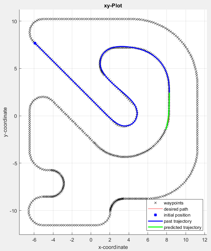
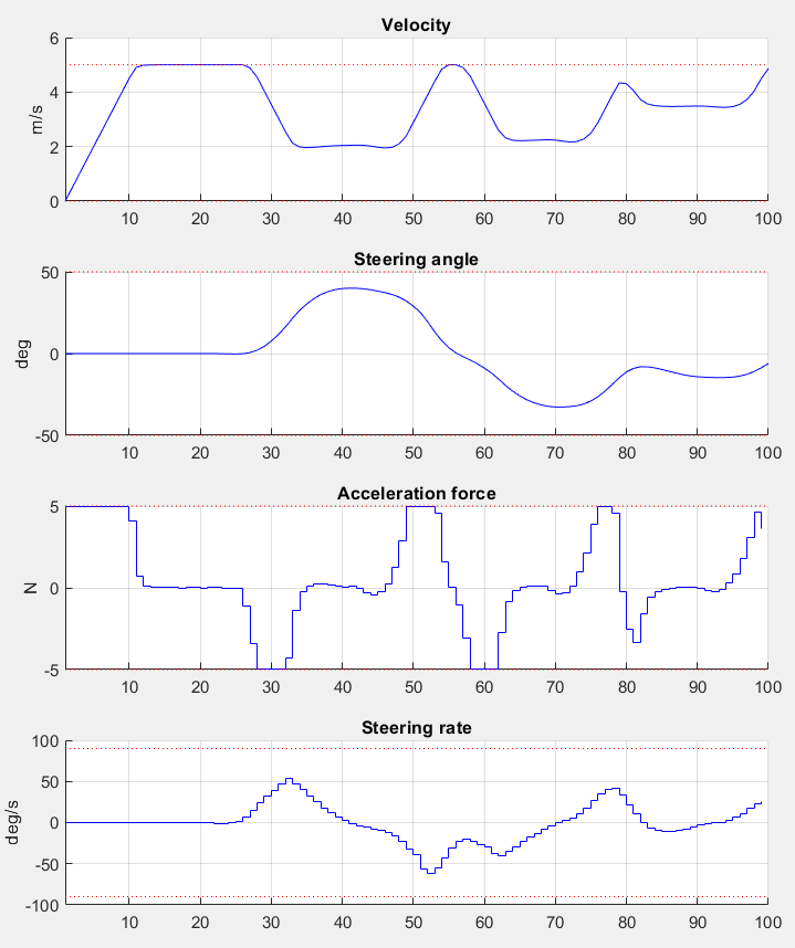
The goal is to find a trajectory that steers the vehicle as close to the provided racetrack waypoints as possible. The trajectory should also be feasible with respect to the vehicle dynamics and its safety and physical limitations. The 2D calculated vehicle’s trajectory at timestep \(k=100\) is presented in blue in Figure 11.36. Here, you can see the current predictions for the trajectory marked green. The progress of the other states and inputs over time as well as their predictions is shown in Figure 11.37.

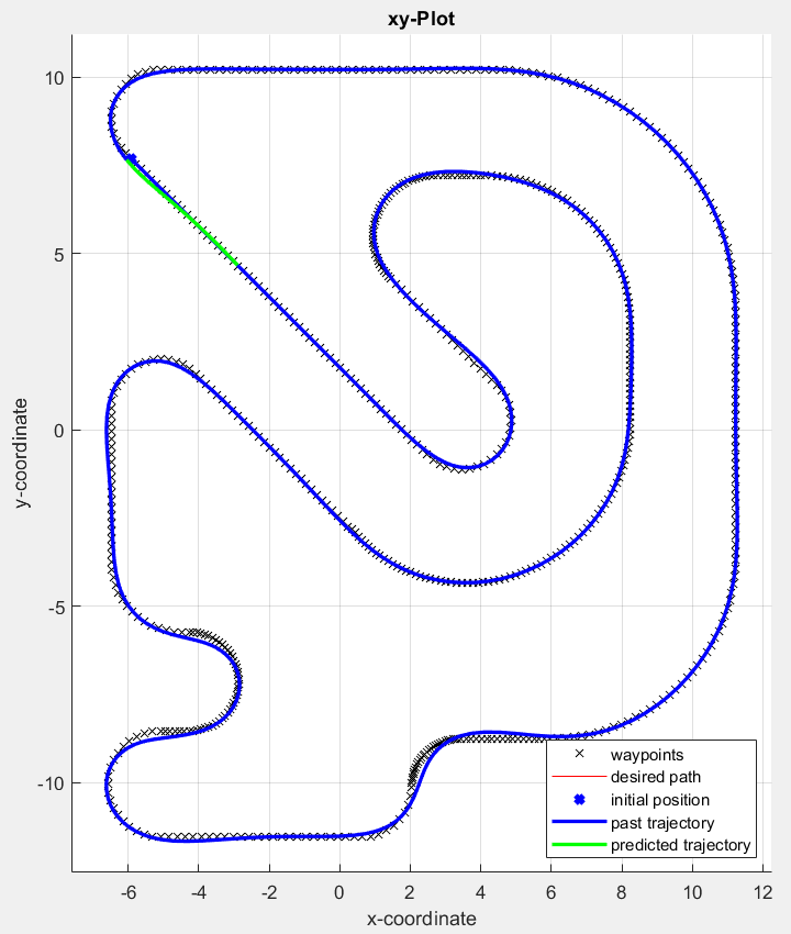
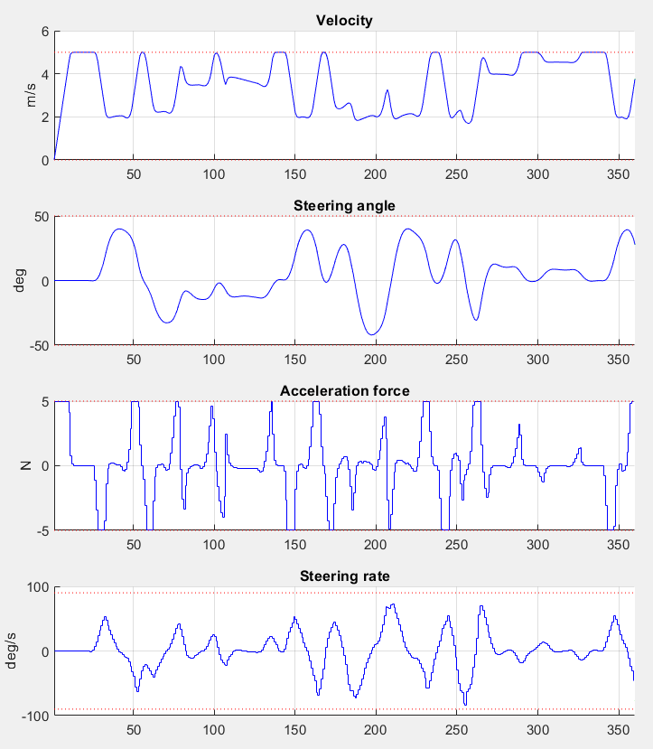
The trajectory and the progress of the system variables over the entire simulation period of 360 steps are presented in Figure 11.38 and Figure 11.39. One can see that all constraints are respected.

To see how the predictions of the system variables develop over all timesteps you can run the example file on your own machine.

Figure 11.36 The calculated trajectory of the car (blue) and its predictions (green) at timestep \(k=100\) (racetrack map from repository https://github.com/alexliniger/MPCC)

Figure 11.37 Development of the vehicle’s states and the system’s inputs over time at timestep \(k=100\)

Figure 11.38 The calculated trajectory of the car (racetrack map from repository https://github.com/alexliniger/MPCC)

Figure 11.39 Development of the vehicle’s states and the system’s inputs over time

11.11.5. Using the SQP Fast solver

The above sections illustrate how to specify a dynamical model and generate a FORCESPRO solver to use in a reference-tracking MPC algorithm. Since FORCESPRO version 6.0.0, FORCESPRO supports a SQP Fast solver (see Tuning the SQP Fast solver). This algorithmic choice changes the workflow a little as it requires the user to tune the solver in order to obtain a solver which is tailored to the specific application. This tuning procedure can be done using the FORCESPRO “autotune” tool (see Autotuner).

You can download a variant of this example with the complete workflow for the SQP Fast solver here.

The key step in tuning a fast SQP solver is to collect problem data on which certain algorithmic parameters are tuned. For this, one generates a solver (with codeoptions.sqp_nlp.qp_method = "general") exactly as above and then performs the simulation in order to save the simulation data (the tuningProblems in the code-snippet in Calling the generated solver). Once this data has been stored a fast SQP solver can be generated and tuned as follows:

Matlab

% Generate fast SQP solver based on a fast QP solver
tuningoptions = ForcesAutotuneOptions(tuningProblems);
ForcesGenerateSqpFastSolver(model, codeoptions, tuningoptions);

Note that the FORCESPRO autotuning tool allows for a great deal of customization. Such customization is specified via the ForcesAutotuneOptions object (see Autotuner Options).