11.14. High-level interface: Soft Constraints
As in section High-level interface: Basic example we consider the following linear MPC problem with lower and upper bounds on state and inputs, and a terminal cost term:
This problem is parametric in the initial state \(\color{red} x\) and the first input \(u_0\) is typically applied to the system after a solution has been obtained. For the sake of this example, we assume \(u_i \in \mathbb{R}\) and \(x_i \in \mathbb{R}^2\) and write
Suppose we want to allow the inequality constraints for \(u_i\) to be slightly violated. In this case, we introduce a slack variable \(s_i \geq 0\) and write
We want to punish positive values of \(s_i\) by adding a penalty term to the objective function. We use a hyperparameter \(\lambda \geq 0\) and write
Here, we use a penalty term linear in \(s_i\). For \(\lambda\) large enough, the slack variables \(s_i\) are only chosen positive
if the problem is infeasible with a hard constraint. For small \(\lambda\), it may be optimal to slightly violate the constraints even though
the original problem is feasible. It is also common to choose a penalty term quadratic in \(s_i\). In order to use the FORCESPRO
framework, we need to recast the new inequality constraints:
with \(h_1(u_i,s_i) = u_i - s_i\) and \(h_2(u_i,s_i) = u_i + s_i\).
11.14.1. Implementation in MATLAB
The following code is based on the MATLAB code in High-level interface: Basic example. The modified inequality constraints can be implemented as follows:
%% relaxed inequality constraints
% assume variable ordering zi = [si, ui, xi]

model.nh    = 2;                     % number of inequality constraints
model.ineq  = @(z) [ z(2) - z(1);    % h_1
                    z(2) + z(1)];   % h_2
model.hu    = [umax, +inf];          % upper bound on inequality constraints
model.hl    = [-inf, umin];          % lower bound on inequality constraints
# relaxed inequalities constraints
# assume variable ordering zi = [si, ui, xi]

model.ineq = lambda z: casadi.vertcat( z[1] - z[0],
                                      z[1] + z[0])
model.hu = np.array([umax, +float('inf')])
model.hl = np.array([-float('inf'), umin])
The resulting code is depicted below.
%% system
A = [1.1 1; 0 1];
B = [1; 0.5];
[nx,nu] = size(B);
lambda = 8; % measure for penalty term

%% MPC setup
Q = eye(nx);
R = eye(nu);
if( exist('dlqr','file') )
    [~,P] = dlqr(A,B,Q,R);
else
    P = 10*Q;
end
umin = -0.5;     umax = 0.5;
xmin = [-5, -5]; xmax = [5, 5];

%% FORCESPRO multistage form
% assume variable ordering z(i) = [si; ui; xi] for i=1...N

% dimensions
model.N     = 11;   % horizon length
model.nvar  = 4;    % number of variables
model.neq   = 2;    % number of equality constraints
model.nh    = 2;    % number of inequality constraints

% objective with penalty term
model.objective = @(z)  z(2)*R*z(2) + [z(3); z(4)]'*Q*[z(3); z(4)] + lambda*z(1);
model.objectiveN = @(z) [z(3); z(4)]'*P*[z(3); z(4)];

% equalities
model.eq = @(z) [ A(1,:)*[z(3); z(4)] + B(1)*z(2);
                  A(2,:)*[z(3); z(4)] + B(2)*z(2)];

model.E = [zeros(2,2), eye(2)];

% initial state
model.xinitidx = 3:4;

% relaxed inequalities
model.ineq = @(z) [ z(2) - z(1);
                    z(2) + z(1)];
model.hu = [umax, +inf];
model.hl = [-inf, umin];


model.lb = [0,      -inf, xmin  ];
model.ub = [+inf,   +inf, xmax  ];
# system
A = np.array([[1.1, 1], [0, 1]])
B = np.array([[1], [0.5]])
nx, nu = np.shape(B)
lam = 8 # measure for penalty term

# MPC setup
N = 10
Q = np.eye(nx)
R = np.eye(nu)
P = 10*Q
umin = -0.5
umax = 0.5
xmin = np.array([-5, -5])
xmax = np.array([5, 5])

# FORCESPRO multistage form
# assume variable ordering zi = [si; ui; xi] for i=0...N

# dimensions
model = forcespro.nlp.ConvexSymbolicModel(11)   # horizon length N+1
model.nvar = 4    # number of variables
model.neq = 2   # number of equality constraints
model.nh = 2

# objective with penalty term
model.objective = (lambda z: z[1]*R*z[1] + lam*z[0] +
                  casadi.horzcat(z[2], z[3]) @ Q @ casadi.vertcat(z[2], z[3]))
model.objectiveN = (lambda z:
                    casadi.horzcat(z[2], z[3]) @ P @ casadi.vertcat(z[2], z[3]))

# equalities
model.eq = lambda z: casadi.vertcat(casadi.dot(A[0, :], casadi.vertcat(z[2], z[3])) + B[0, :]*z[1],
                              casadi.dot(A[1, :], casadi.vertcat(z[2], z[3])) + B[1, :]*z[1])

model.E = np.concatenate([np.zeros((2, 2)), np.eye(2)], axis=1)

# initial state
model.xinitidx = [2, 3]

# relaxed inequalities
model.ineq = lambda z: casadi.vertcat( z[1] - z[0],
                                      z[1] + z[0])
model.hu = np.array([umax, +float('inf')])
model.hl = np.array([-float('inf'), umin])

# inequalities
model.lb = np.concatenate([[0, -float('inf')], xmin])
model.ub = np.concatenate([[float('inf'), float('inf')], xmax])
You can download the code of this example to try it out for yourself:
MATLAB,
PYTHON.
11.14.2. Results
We run the simulation for \(\lambda = 2, 8\). The results of the simulation are presented in Figure 11.46 below. The plot on the top shows the system’s states over time, the plot on the bottom shows the input commands. For \(\lambda = 2\), the constraints on \(u\) are clearly violated, for \(\lambda = 8\), these constraints are only slightly violated.
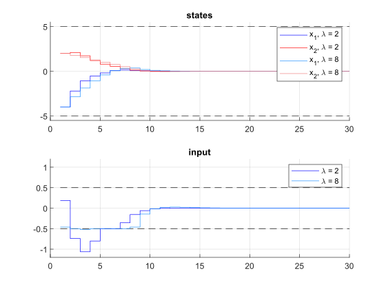
Figure 11.46 Simulation results of the states (top), input (middle) over time. The constraints are plotted in black dashed lines.